BBP Strong Ground Motion Project

Southern California Plate Boundary (SCPB) Velocity Model

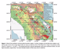
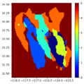
The Fang et al paper defines a Southern California Plate Boundary Velocity model. The max depth is 20 km; the model should be merged with a regional model to have information below that depth but this will require smoothing between models. We are looking at the Vp, Vs models of the Fang et al. (2016) pape. , and also the Fang et al. (GJI, 216, 609–620, doi: 10.1093/gji/ggy458.2019) paper that has better Vs results, and classify the results using K-means clusters as done by Eymold and Jordan (2019). We found that 6 clusters (data types) can account for most of the data. This is preliminary but can help to decide how many distinct 1D velocity models are needed for the region around the SJFZ. More work is required to decide how to merge the results with a regional model.

The horizontal grid spacing in Fang et al. (2106) has an interval of 0.03 deg in both latitude and longitude, which is about 3.3 km. The damage zones results from Allam and Ben-Zion (2012) and also Zigone et al. (2015) are included in the joint inversions of Fang et al. (2016, 2019). The image above shows the main clusters of velocity models Hao created from the Vp,Vs models of Fang et al. We are checking if the fault damage zones are already represented (if not they can be added by increasing the number of clusters).

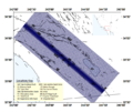
The horizontal spacing of the nodes in the Allam and Ben-Zion 2012 is variable, starting with 100 m around the SJFZ (see brief text below and attached figure). This fine grid does not mean a resolution of 100 m around the fault, but a resolution of 1 km is a first order estimate.

The model was developed by solving for P-wave velocities (Vp) and earthquake locations on a uniform 1 km-spaced grid using a smoothed 1-D starting model (Fig. 2a) derived from Helmberger et al. (1992). The obtained velocities and event locations are then used iteratively as initial values for inversions on a variable grid that is progressively reduced to a minimum spacing of 100 m in the 4.5 km region on each side (y direction) of the SJFZ. The grid cells in the x and z directions remain uniformly spaced at 1 km. A more detailed discussion of the inversion grid and MATLAB code for generating it are included in Appendix B; a geographical location map for the grid points used is shown in Fig. S1 (above).

Prototype Web viewer for SCPB Velocity Model

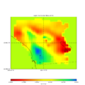
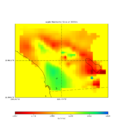
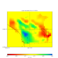
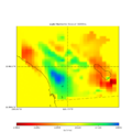
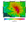
This web viewer can create vertical profiles and cross section plots of the Fang et all SCPBVM. The images below show how the webviewer reproduces the images from Fang et all (2016) Fig. 3 at depths 3km, 7km, 11km, and 16km.

SCPBVM Web Viewer

Horizontal Cross Sections Plots of the SCPB Velocity Model

This web viewer can create vertical profiles and cross section plots of the Fang et all SCPB Velocity Model. The images below show how the webviewer reproduces the images from Fang et all (2016) Fig. 3 at depths 3km, 7km, 11km, and 16km.

Full Resolution Model

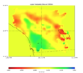
Vs 3km
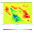
Vs 7km
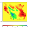
Vs 11km
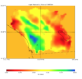
Vs 16km

Downsampled Model

Vs 3km
Vs 7km
Vs 11km
Vs 16km

[[Image:Fang_Fig3_vs.png|none|300px]|Fang et al Fig 3 Vs profiles]

Velocity Model Figures

SCPB Velocity Model Map
Sensor Net Distribution
So. Calif Velocity Regions

Related Papers and Datasets

Model Data File

Fang SCPB velocity model data files

The model data folder has Vp, Vs, and the geographic coordinates. The format is defined as:


X1Y1Z1 X2Y1Z1 ... X1Y1Z1
X1Y2Z1 ...
.
.
X1Y1Z2 ...
.
.
X1YNZN ...

AGU Abstract

Evaluating the Impact of Alternative Seismic Velocity Models on Simulated Ground Motions from Large Magnitude California Earthquakes

Philip J. Maechling, Fabio Silva, Robert Graves and Yehuda Ben-Zion

Ground motion simulation methods implemented in the SCEC Broadband Platform (BBP) are designed to simulate strong ground motions at levels of engineering interest. The simulation methods have undergone extensive verification and validation efforts involving comparison of simulated results to Ground Motion Prediction Equations (GMPEs) and to the observed ground motions from historical earthquakes. The ground motion simulation methods implemented in the platform propagate seismic waves through a region-specific 1D velocity model, and typically a single 1D velocity model is selected for each validation earthquake. Recently, dense seismic arrays and other methods have produced detailed velocity models for Southern California that often resolve near surface layers better than earlier models. The goal of this study is to use the BBP with multiple 1D velocity models in a region, to study the impact of the different velocity models on the simulated ground motions. We use the Graves and Pitarka ground motion method as implemented in the BBP and large scenario earthquakes on the San Jacinto Fault and the Newport Inglewood Fault consistent with high probability UCERF3 ruptures for Southern California. Initial results in comparison with baseline ground motions using the existing BBP region-specific 1D velocity models will be presented in the meeting.

Creating PGA/PGV Maps

In order to create PGA/PGV maps, we follow the steps below.

Landers Multi-Segment

Landers MS (PGV)
Landers MS Station Map

Generating station grid

For Landers, we use a station grid from 33.4 to 35.9 latitude, and -115 to -119.2 longitude, spaced at 0.1 degrees of latitude and longitude:

$ gen_station_grid.py  33.4 35.9 -119.2 -115 .1 > landers_01_grid.stl

Including Vs30 values

Once the station list is generated, we need to include Vs30 values. We use the SiteData GUI application from opensha-apps.

$ java -jar SiteDataGUI-2022_07_27-afbf611e.jar

Then, select

CGS/Wills VS30 Map (2015)
Global Vs30 from Topographic Slope (Wald & Allen 2008)

The Global Vs30 values will be used for water (value set to 180 m/s) and for Nevada (which is not included in the Wills 2015 map.

Running BBP Simulation

The next step is to run the BBP at CARC/USC. We use the SRC files from the Landers and/or Landers Multi-Segment validation package(s), which is included with BBP 22.4. To create the CARC runs, users can use one of the following two commands (for the single-segment, or the multi-segment version of Landers):

$ bbp_discovery_split_scenario.py -c gp --email=fsilva@usc.edu -v Mojave500 --src=landers_v20_07_1.src --stl=landers_01_grid_vs30_full.stl -s gp -n 30 -d landers-mojave-ss

$ bbp_discovery_split_scenario.py -c gp --email=fsilva@usc.edu -v Mojave500 --src="landers_v16_08_1_seg1.src, landers_v16_08_1_seg2.src, landers_v16_08_1_seg3.src" --stl=landers_01_grid_vs30_full.stl -s gp -n 30 -d landers-mohave-ms

The commands above will split the simulation into several realizations, which all use the same SRC file, but each include a subset of 30 stations from the original station list. This shares the processing among several CPUs and allows the simulation to complete quickly. Once the simulations finish, we need to merge the realizations in to a single realization (we picked the number 2 for the realization sim_id):

$ bbp_merge_scenario.py -d landers-mojave-ms -s 2

$ bbp_merge_scenario.py -d landers-mojave-ss -s 2

Collecting and Processing PGA/PGV Data

The next step is to collect PGA and PGV data from each of the stations. We can use the get_shakemap_data script that is included with the BBP 22.4 distribution:

$ get_shakemap_data.py landers-mojave-ms/Sims/indata/2/landers_01_grid_vs30_full.stl landers-mojave-ms/Sims/outdata/2 pgv-log > landers-mojave-ms-2022-08-11-pgv-log

$ get_shakemap_data.py landers-mojave-ms/Sims/indata/2/landers_01_grid_vs30_full.stl landers-mojave-ms/Sims/outdata/2 pga-log > landers-mojave-ms-2022-08-11-pga-log.txt

$ get_shakemap_data.py landers-mojave-ms/Sims/indata/2/landers_01_grid_vs30_full.stl landers-mojave-ms/Sims/outdata/2 pga-g > landers-mojave-ms-2022-08-11-pga-g.txt

$ get_shakemap_data.py landers-mojave-ss/Sims/indata/2/landers_01_grid_vs30_full.stl landers-mojave-ss/Sims/outdata/2 pgv-log > landers-mojave-ss-2022-08-11-pgv-log.txt

$ get_shakemap_data.py landers-mojave-ss/Sims/indata/2/landers_01_grid_vs30_full.stl landers-mojave-ss/Sims/outdata/2 pga-log > landers-mojave-ss-2022-08-11-pga-log.txt

$ get_shakemap_data.py landers-mojave-ss/Sims/indata/2/landers_01_grid_vs30_full.stl landers-mojave-ss/Sims/outdata/2 pga-g > landers-mojave-ss-2022-08-11-pga-g.txt

And the following commands swap the longitude/latitude values, as expected by the OpenSHA plotting tool:

$ cat landers-mojave-ss-2022-08-11-pgv-log.txt | awk '{ print $2 " " $1 " " $3 }' > landers-mojave-ss-2022-08-11-pgv-log-results.txt

$ cat landers-mojave-ms-2022-08-11-pgv-log.txt | awk '{ print $2 " " $1 " " $3 }' > landers-mojave-ms-2022-08-11-pgv-log-results.txt

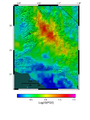
Generating PGA/PGV Maps

We use the GMTMapApp tool from OpenSHA:

$ java -jar GMTMapApp-2022_08_10-253cf2c3.jar

For Landers, we pick the following parameters:

Min Latitude: 33.4
Max Latitude: 35.8
Min Longitude: -119.2
Max Longitude: -115.0
Grid Spacing: 0.1
Color Scheme: MaxSpectrum.cpt
Color Scale Limits: Manually
Color Scale Min: -0.02
Color Scale Max: 1.95
Topo Resolution: 03 sec California
Highways: None
Coast: Draw & Fill
Image Width: 6.5
Custom Scale Label: Checked
Scale Label: Log10(PGV)
Apply GMT Smoothing: Checked
Apply Black Background: Not checked
DPI: 300
Plot Log: Not checked
Generate KML Files: Not checked
Use grdview instead of grdimage: Not checked

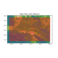
Plot Station Maps

The last step is to generate the station maps with rupture trace:

$ cp ../landers-mojave-ss/Sims/indata/10000000/landers_v20_07_1-gp-0000.srf indata/2/
$ cp ../landers-mojave-ms/Sims/indata/10000000/landers_v16_08_1_seg1-gp-0000_seg01.srf indata/3/
$ cp ../landers_01_grid_vs30_full.stl  indata/2/.
$ cp ../landers_01_grid_vs30_full.stl  indata/3/.
$ $BBP_DIR/comps/plot_map.py landers_v20_07_1-gp-0000.srf landers_01_grid_vs30_full.stl 2
$ $BBP_DIR/comps/plot_map.py landers_v16_08_1_seg1-gp-0000_seg01.srf landers_01_grid_vs30_full.stl 3

Ridgecrest 2019C Multi-Segment

Ridgecrest-19CMS (PGV)
Ridgecrest-19CMS Station Map

Generating station grid

For Ridgecrest 2019C, we use a station grid from 33.4 to 36.9 latitude, and -116 to -119.2 longitude, spaced at 0.1 degrees of latitude and longitude:

$ gen_station_grid.py  33.4 36.9 -119.2 -116 .1 > ridgecrest_grid.stl

Including Vs30 values

Once the station list is generated, we need to include Vs30 values. We use the SiteData GUI application from opensha-apps.

$ java -jar SiteDataGUI-2022_07_27-afbf611e.jar

Then, select

CGS/Wills VS30 Map (2015)
Global Vs30 from Topographic Slope (Wald & Allen 2008)

The Global Vs30 values will be used for water (value set to 180 m/s) and for Nevada (which is not included in the Wills 2015 map.

Running BBP Simulation

The next step is to run the BBP at CARC/USC. We use the SRC files from the Ridgecrest 2019C validation package, which is included with BBP 22.4. To create the CARC runs, users can use one of the following command:

$ bbp_discovery_split_scenario.py -c gp --email=fsilva@usc.edu -v SouthernSierra500-2 --src="ridgecrest-c_v20_09_1_seg1.src, ridgecrest-c_v20_09_1_seg2.src, ridgecrest-c_v20_09_1_seg3.src" --stl=ridgecrest_grid_basic.stl -d ridgecrest19c-ms -n 30 -s gp

The command above will split the simulation into several realizations, which all use the same SRC file, but each include a subset of 30 stations from the original station list. This shares the processing among several CPUs and allows the simulation to complete quickly. Once the simulations finish, we need to merge the realizations in to a single realization (we picked the number 2 for the realization sim_id):

$ bbp_merge_scenario.py -d ridgecrest19c-ms -s 2

Collecting and Processing PGA/PGV Data

The next step is to collect PGA and PGV data from each of the stations. We can use the get_shakemap_data script that is included with the BBP 22.4 distribution:

$ get_shakemap_data.py ridgecrest19c-ms/Sims/indata/2/ridgecrest_grid_basic.stl ridgecrest19c-ms/Sims/outdata/2 pgv-log > ridgecrest19c-ms-2022-08-11-pgv-log.txt

$ get_shakemap_data.py ridgecrest19c-ms/Sims/indata/2/ridgecrest_grid_basic.stl ridgecrest19c-ms/Sims/outdata/2 pga-log > ridgecrest19c-ms-2022-08-11-pga-log.txt

$ get_shakemap_data.py ridgecrest19c-ms/Sims/indata/2/ridgecrest_grid_basic.stl ridgecrest19c-ms/Sims/outdata/2 pgv-g > ridgecrest19c-ms-2022-08-11-pgv-g.txt

And the following command swaps the longitude/latitude values, as expected by the OpenSHA plotting tool:

$ cat ridgecrest19c-ms-2022-08-11-pgv-log.txt | awk '{ print $2 " " $1 " " $3 }' > ridgecrest19c-ms-2022-08-11-pgv-log-results.txt

Generating PGA/PGV Maps

We use the GMTMapApp tool from OpenSHA:

$ java -jar GMTMapApp-2022_08_10-253cf2c3.jar

For Ridgecrest 19C, we pick the following parameters:

Min Latitude: 33.4
Max Latitude: 36.8
Min Longitude: -119.2
Max Longitude: -116.0
Grid Spacing: 0.1
Color Scheme: MaxSpectrum.cpt
Color Scale Limits: Manually
Color Scale Min: 0.01
Color Scale Max: 2.05
Topo Resolution: 03 sec California
Highways: None
Coast: Draw & Fill
Image Width: 6.5
Custom Scale Label: Checked
Scale Label: Log10(PGV)
Apply GMT Smoothing: Checked
Apply Black Background: Not checked
DPI: 300
Plot Log: Not checked
Generate KML Files: Not checked
Use grdview instead of grdimage: Not checked

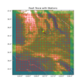
Plot Station Maps

The last step is to generate the station maps with rupture trace:

$ cp ../ridgecrest19c-ms/Sims/indata/10000000/ridgecrest-c_v20_09_1_seg1-gp-0000_seg01.srf indata/1
$ cp ../ridgecrest_grid_final.stl  indata/1/.
$ $BBP_DIR/comps/plot_map.py ridgecrest-c_v20_09_1_seg1-gp-0000_seg01.srf ridgecrest_grid_final.stl 1

BBP Strong Ground Motion Project

Contents

Southern California Plate Boundary (SCPB) Velocity Model

Prototype Web viewer for SCPB Velocity Model

Horizontal Cross Sections Plots of the SCPB Velocity Model

Velocity Model Figures

Related Papers and Datasets

Model Data File

AGU Abstract

Creating PGA/PGV Maps

Landers Multi-Segment

Generating station grid

Including Vs30 values

Running BBP Simulation

Collecting and Processing PGA/PGV Data

Generating PGA/PGV Maps

Plot Station Maps

Ridgecrest 2019C Multi-Segment

Generating station grid

Including Vs30 values

Running BBP Simulation

Collecting and Processing PGA/PGV Data

Generating PGA/PGV Maps

Plot Station Maps

Related Entries

Navigation menu

Page actions

Page actions

Personal tools

Navigation

Search

Tools