CyberShake Study 15.12
CyberShake Study 15.12 takes the deterministic results from CyberShake Study 15.4 and adds broadband components.
Contents
Status
Study 15.12 began production at 19:59:54 PST on December 3, 2015. Estimated completion is February 29, 2016.
Computational Goal
We are working on doing a series of broadband CyberShake runs, extending the 1 Hz deterministic results we generated in the spring with stochastic results from high-frequency implementation on the BBP.
Before we setup the calculation, we evaluate questions about the 1D velocity model needed for the high frequency results. It seems like there are three ways we could handle this in the context of CyberShake:
- Use the same model (LA Basin?) for all CyberShake sites and all ruptures.
- Select the model based on the CyberShake site, and use the same model for all ruptures on that site.
- Select the model based on the rupture, and use the same model for all sites which include that rupture.
Development Approach
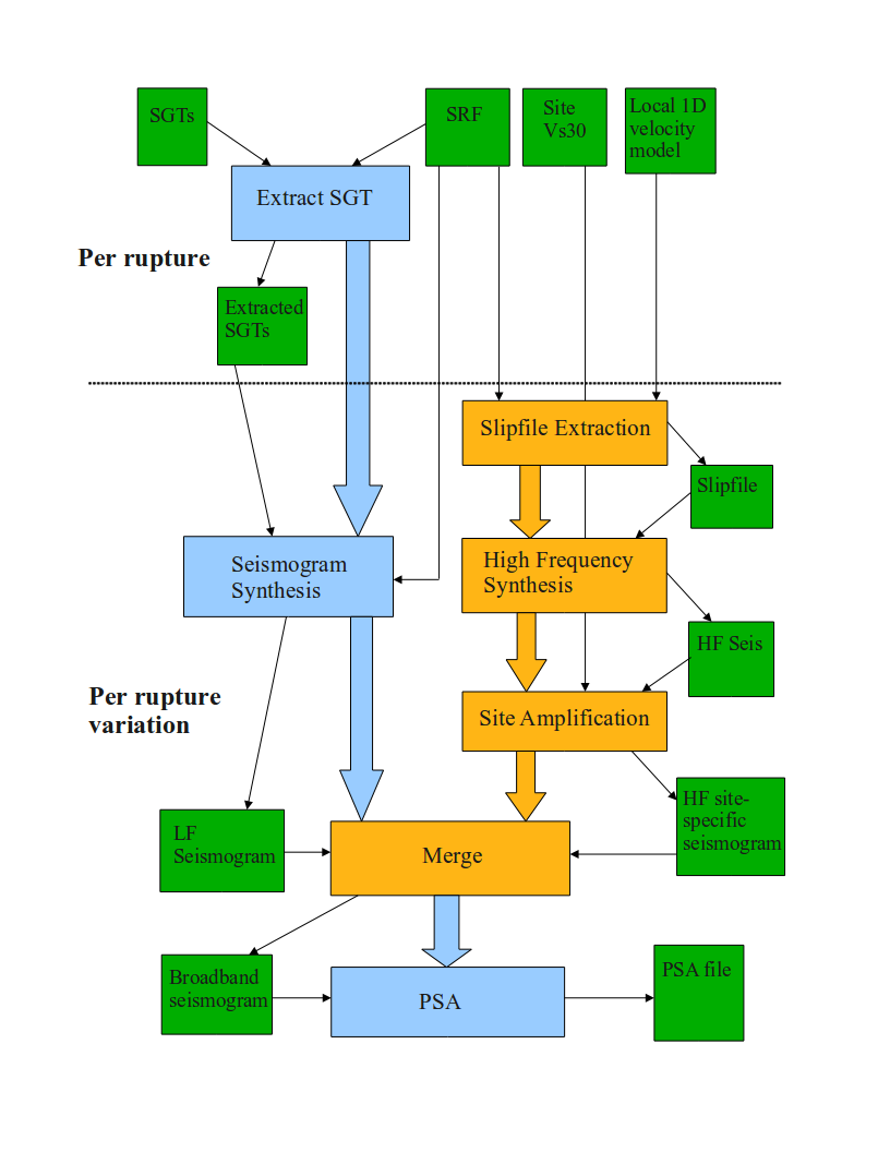
Begin work on a software prototype in which we combine CyberShake 15.4 1Hz CyberShake seismograms with GP BBP High Frequencies, to produce Broadband CyberShake Seismograms. For each site, we expect to take each CyberShake rupture variation, retrieve the SRF used, and the 1Hz seismograms produced, and then run the most recent BBP GP high frequency codes, and merge the HF with the 1Hz CyberShake LF, and produced BBP CyberShake seismograms. We will try to show, using a limited number of sites, we get usable BBP seismograms results. Eventually, we may add the BBP HF processing to the CyberShake platform, and routine produce both 1Hz and BBP seismograms and amplitude data sets.
Technical Approach
There are specific details here and it has to do with the way site-response is handled for the high frequencies.
The current BBP is set-up for computing ground motions at a "hard-rock" site, typically Vs30=865 m/s. (The reason behind this seemingly random value is that the site-response module in GP2010 used the Campbell-Bozorgnia amplification factors, which are linear functions for Vs30 >= 865 m/s.)
To compute the high-frequency motions for sites with Vs30 < 865 m/s, it is not as straightforward as simply replacing the prescribed 1D velocity structure with something that has lower velocities in the near surface. The problem is that the HF simulation codes on the BBP do not model non-linear behavior. GP2010 addressed this by using a post-processing step that applied empirically-based, frequency-dependent, non-linear amplification factors to adjust the computed rock-site motions to a (presumably lower) site-specific Vs30 value. The codes to do this are in the BBP source code distribution("wcc_siteamp"). However, they were not used for any of the validation exercises since those were all hard-rock based, and the BBP scripts probably have had any references to these codes deleted or commented out.
Our Proposed method on how to proceed for CyberShake is as follows:
- Use a single 1D velocity profile for all LA area sites that is "hard-rock". The Northridge 1D model
(with Vs30=865 m/s) that is already on the BBP is the current preferred choice.
- For "rock" sites, the HF and LF results could be combined and used as is.
- For sites with Vs30 lower than about 600-700 m/s, the HF results should be modified to account for site-specific ground motion response. This should be done to the HF motions prior to combining with the LF response. At this point, we will not make any type of modification to the LF motions, for soft soil sites, although we can reconsider that decision in the future.
Computational Details
A copy of BBP v15.4 is installed on Blue Waters; /u/sciteam/scottcal/scratch/bbp/15.3.0/bbp/src/gp/WccFormat/Progs In the recent BBP install, find it under <version#>/bbp/src/gp/WccFormat/Pros
We confirmed the version of CVM-S4.26 used for CyberShake Study 15.4 does include the GTL, with a 500 m/s minimum cutoff. It sounds like it would be better to extract Vs30 values from it rather than Wills. Should we apply the 500 m/s cutoff to the Vs30 values we pass to site response like we did with CyberShake, or use them as-is?
Site response module: wcc_siteamp. The current version of the code uses site amplification factors based on the 2014 NGA GMPEs. Check to see if that is on the BBP. This version is not formally validated this version (e.g. by redoing the GP2010 validations).Need to make sure to run some compatibility checks just to make sure the results looked OK.
Should we only do it if the Vs30 for the site is below 600-700 m/s.
Apply the modification to all sites without worrying about the specific Vs30. For sites that have Vs30 greater than about 600-700 the modification will be very minor. But the extra overhead in running the code for all sites is probably insignificant relative to the (equally trivial) overhead in checking the sites for an arbitrary Vs30 threshold and having different processing streams based on this.
Related question - in 2011 we pulled the Vs30 values from Wills. Is that still correct, or should we use Vs30 from the velocity model we used for the CyberShake deterministic (CVM-S4.26)?
There are some concerns about the near-surface velocity values in the CVM used for the previous calcualtions, in particular, very high Vs for rock sites, and that is why we used Wills In CVM-S4.26, does it include the "geotechnical layer"? If so, then its probably best to use these values, so that the LF and HF portions are consistent.
Program Name: wcc_siteamp14.c
The input and output are the same as previous versions with the possible exception being the parameter "model". If "model" is not specified, then the default settings are used, which is fine.
Check to see if this parameter was set previously. (i.e., as model=<something> either in a parfile or on the command line)
Regarding the question of whether we should we apply the 500 m/s cutoff to the Vs30 values we pass to site response like we did with CyberShake, or use them as-is? Current decision is to use them as is. There will be an apparent disconnect with the 500 m/s cutoff at some sites, although the the 500 m/s value with a 100 meter grid spacing is an adequate approximation for the LF calculation.
Priority CyberShake Sites of Interest
Broadband-Cybershake motions for a few sites combining the stochastic and Cybershake signals:
- STNI - basin site
- LADT - basin site
- PAS - rock site
- WNGC - between basins, with expected high ground motions
- LADP - another rock site, near fault
BBP CyberShake Schematic 2009
Initial tests
We performed initial tests by using the Graves code from the current version of the BBP to synthesize stochastic seismograms, along with applying site amplification from CB2014. We used the Vs30 value taken from the same velocity model as the deterministic seismograms (CVM-S 4.26). We also applied site amplification from CB2014 to the deterministic seismograms. Then the deterministic seismograms were low-pass filtered at 1.0 Hz, and the stochastic seismograms were high-pass filtered at 1.0 Hz, and the results were combined. From this broadband seismogram we calculated PSA and RotD values.
| Run | 10 sec SA | 5 sec SA | 3 sec SA | 2 sec SA | 1 sec SA | 0.5 sec SA | 0.2 sec SA | 0.1 sec SA |
|---|---|---|---|---|---|---|---|---|
| PAS, broadband (run 4266) | ||||||||
| PAS, broadband (run 4266, blue) vs deterministic (run 3878, black) | ||||||||
| LADT, broadband (run 4271) | ||||||||
| LADT, broadband (run 4271, blue) vs deterministic (run 3870, black) |


Sample Seismogram
Below is a seismogram for PAS, source 273, rupture 69, rupture variation 50, comparing the 1 Hz seismogram (blue) to the 10 Hz seismogram (green). Mostly, the 10 Hz seismogram looks sharper.


Deterministic Site Amplification
We ran PAS and LADT with and without deterministic site amplification (using CB 2014, and Vs30 values from CVM-S4.26, "V1.0"). Here are the results:
| Run | 10 sec SA | 5 sec SA | 3 sec SA | 2 sec SA | 1 sec SA | 0.5 sec SA | 0.2 sec SA | 0.1 sec SA |
|---|---|---|---|---|---|---|---|---|
| PAS, site amplification (run 4266, blue) vs no deterministic site amplification (run 4270, black) | ||||||||
| LADT, site amplification (run 4271, blue) vs no deterministic site amplification (run 4272, black) |


Vs values v2.0
For the stochastic, we continued to use vref=865, and changed to Vs30 = 30 / Sum (1/(Vs sampled from [0.5,29.5] in 1 meter increments)).
For the deterministic, we switched to use vref = Vs @ Z=0 * Vs30 / Vs50 (50 is half the grid spacing of 100m).
For PAS, this means the LF vref went from 865 to 422.4, and the Vs30 went from 821.3 to 838.8.
For LADT, this means the LF vref went from 865 to 436.1, and the Vs30 went from 359.1 to 365.4.
Here are comparison curves for PAS and LADT.
| Run | 10 sec SA | 5 sec SA | 3 sec SA | 2 sec SA | 1 sec SA | 0.5 sec SA | 0.2 sec SA | 0.1 sec SA |
|---|---|---|---|---|---|---|---|---|
| PAS, previous site amp (run 4266, blue) vs new deterministic site amp (run 4275, black) | ||||||||
| LADT, previous site amp (run 4271, blue) vs new deterministic site amp (run 4276, black) |


Vs values v3.0
We modified the vref calculation further, to:
vref_LF_eff = Vs30 * [ VsD5H / Vs5H ]
with Vs30 determined from the CVM as before (averaging over 1 meter increments). The other parameters are determined based on the grid spacing used in the calculation, given by H:
Vs5H = travel time averaged Vs computed from CVM in 1 meter increments down to a depth of 5*H VsD5H = discrete travel time averaged Vs computed from 3D velocity mesh used in the SGT calculation over the upper 5 grid points
So, for H=100m Vs5H would be:
Vs500 = 500 / ( Sum ( 1 / Vs sampled from [0.5,499.5] in 1 meter increments ))
And then VsD5H is given by:
VsD500 = 5/{ 0.5/Vs(Z=0m) + 1/Vs(Z=100m) + 1/Vs(Z=200m) + 1/Vs(Z=300m) + 1/Vs(Z=400m) + 0.5/Vs(Z=500m) }
This gives vref = 705 for PAS, 361 for LADT, and 294 for STNI.
| Run | 10 sec SA | 5 sec SA | 3 sec SA | 2 sec SA | 1 sec SA | 0.5 sec SA | 0.2 sec SA | 0.1 sec SA |
|---|---|---|---|---|---|---|---|---|
| PAS, V1.0 site amp (run 4266, blue) vs V3.0 deterministic site amp (run 4279, black) | ||||||||
| PAS, no deterministic site amp (run 4270, blue) vs V3.0 deterministic site amp (run 4279, black) | ||||||||
| LADT, V1.0 site amp (run 4271, blue) vs V3.0 deterministic site amp (run 4280, black) | ||||||||
| LADT, no deterministic site amp (run 4272, blue) vs V3.0 deterministic site amp (run 4280, black) | ||||||||
| STNI, 1 Hz deterministic (run 3873, blue) vs V3.0 deterministic site amp (run 4281, black) |


srf2stoch_lite
To reduce the memory requirements of srf2stoch, Rob Graves created a new version, srf2stoch_lite, with much smaller memory requirements. The differences in hazard curves can be seen here, for PAS. Since srf2stoch is only used in the high frequency, we are only looking at high frequency curves. Blue is with srf2stoch, black is with srf2stoch_lite.
| 2 sec | 1 sec | 0.5 sec | 0.2 sec | 0.1 sec | |
|---|---|---|---|---|---|
| Curve | |||||
| Avg absolute % diff | 0.4% | 1.9% | 1.7% | 33.9% (skewed by 1 point; otherwise it's 1.8%) |
2.7% |
| Max % diff | 8.4%, at x=0.50g | 29.6%, at x=1.58g | 34.3%, at x=3.98g | 1448.7%, at x=2.51g | 68.4%, at x=2.00g |


