Difference between revisions of "CVM-S5"
(Redirected page to CVM-S4.26) |
|||
| (21 intermediate revisions by 2 users not shown) | |||
| Line 1: | Line 1: | ||
| + | #redirect [[CVM-S4.26]] | ||
== Community Velocity Model - SCEC 5 == | == Community Velocity Model - SCEC 5 == | ||
| − | CVM-S5 is an improved version of the CVM-S4 velocity model which includes full 3D tomographic improvements to the SCEC 4 velocity model as well as an optional GTL implementation. | + | CVM-S5 is an improved version of the CVM-S4 velocity model which includes full 3D tomographic improvements to the SCEC 4 velocity model as well as an optional GTL implementation. Please note that unlike CVM-S4.26, CVM-S5 does not "merge" the results of the inversion with an underlying velocity model. Therefore it is strictly the 26th iteration dataset, 500m resolution, tri-linearly interpolated. There is no background model included, although UCVM can tile a background 1D model should the user specifically ask for it. |
| + | |||
| + | == CyberShake Histogram Plots == | ||
| + | |||
| + | === Vs30 at CyberShake Sites === | ||
| + | |||
| + | {| | ||
| + | |[[File:Cvms5_vs30.png|500px]] | ||
| + | |[[File:Cvms4_vs30.png|500px]] | ||
| + | |- | ||
| + | |[[File:Cvmh_vs30.png|500px]] | ||
| + | |} | ||
| + | |||
| + | === Z1.0 at CyberShake Sites === | ||
| + | |||
| + | {| | ||
| + | |[[File:Cvms5_z10.png|500px]] | ||
| + | |[[File:Cvms4_z10.png|500px]] | ||
| + | |- | ||
| + | |[[File:Cvmh_z10.png|500px]] | ||
| + | |} | ||
| + | |||
| + | === Z2.5 at CyberShake Sites === | ||
| + | |||
| + | {| | ||
| + | |[[File:Cvms5_z25.png|500px]] | ||
| + | |[[File:Cvms4_z25.png|500px]] | ||
| + | |- | ||
| + | |[[File:Cvmh_z25.png|500px]] | ||
| + | |} | ||
| + | |||
| + | == Material Properties Below 50km == | ||
| + | |||
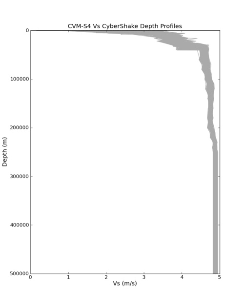
| + | The image below shows depth profiles for all CyberShake sites plotted onto one image. The depth goes from 0km to 500km. | ||
| + | |||
| + | [[File:Cvms4_vs_cybershake_500km.png|500px]] | ||
| + | |||
| + | In the two images below, CVM-S5 is in red and CVM-S4 is in blue. Currently, CVM-S5 returns the material properties at 50km for all depths below 50km. | ||
| + | |||
| + | {| | ||
| + | |[[File:usc500km.png|500px]] | ||
| + | |[[File:perris500km.png|500px]] | ||
| + | |} | ||
| + | |||
| + | == Attenuation Relationship == | ||
| + | |||
| + | Attenuation is based off of Olsen et al., 2003 and is calculated as follows: | ||
| + | |||
| + | If Vs < 1500:<br /> | ||
| + | Qs = Vs * 0.02<br /> | ||
| + | Else:<br /> | ||
| + | Qs = Vs * 0.10 | ||
| + | |||
| + | Qp = Qs * 1.5 | ||
| + | |||
| + | == Density Based on Vs == | ||
| + | |||
| + | According to Po Chen: | ||
| + | |||
| + | "The Vs-density relation was obtained from Table 1 in Brocher 2005. In that table, the 3rd column is Vs and the 5th column is density. So I did a regression using data from these two columns and obtained a polynomial relation for Vs-density. Those numbers in that data file are the coefficients of the polynomial." | ||
| + | |||
| + | The actual polynomial is: | ||
| + | |||
| + | 1.2948318548300342 + 1.2550758337054457Vs - 0.51231936640441489Vs<sup>2</sup> + 0.051962399479341816Vs<sup>3</sup> + 0.015600987888334450Vs<sup>4</sup> - 0.0024189659303912917Vs<sup>5</sup> | ||
== Initial Plots == | == Initial Plots == | ||
| + | |||
| + | === CVM-S5 0m to 500m with GTL === | ||
| + | |||
| + | {| | ||
| + | |[[File:Cvms5_horizontal_0_gtl.png|500px]] | ||
| + | |[[File:Cvms5_horizontal_100_gtl.png|500px]] | ||
| + | |- | ||
| + | |[[File:Cvms5_horizontal_200_gtl.png|500px]] | ||
| + | |[[File:Cvms5_horizontal_300_gtl.png|500px]] | ||
| + | |- | ||
| + | |[[File:Cvms5_horizontal_400_gtl.png|500px]] | ||
| + | |[[File:Cvms5_horizontal_500_gtl.png|500px]] | ||
| + | |} | ||
| + | |||
| + | === Depth Profiles === | ||
| + | |||
| + | ==== Surface Profiles ==== | ||
| + | |||
| + | {| | ||
| + | |Del Amo -118.09624, 33.84822<br />[[File:delamo_cvms5.png|500px]] | ||
| + | |Diablo Canyon -120.85611, 35.21083<br />[[File:diablocanyon_cvms5.png|500px]] | ||
| + | |- | ||
| + | |PERRIS -117.24904, 3380594<br />[[File:perris_cvms5.png|500px]] | ||
| + | |USC -118.286, 34.0192<br />[[File:usc_cvms5.png|500px]] | ||
| + | |} | ||
| + | |||
| + | ==== 60km Profiles ==== | ||
| + | |||
| + | {| | ||
| + | |Del Amo -118.09624, 33.84822<br />[[File:delamo_cvms5_60km.png|500px]] | ||
| + | |Diablo Canyon -120.85611, 35.21083<br />[[File:diablo_canyon_cvms5_60km.png|500px]] | ||
| + | |- | ||
| + | |PERRIS -117.24904, 3380594<br />[[File:perris_cvms5_60km.png|500px]] | ||
| + | |USC -118.286, 34.0192<br />[[File:usc_cvms5_60km.png|500px]] | ||
| + | |} | ||
| + | |||
=== CVM-S5 0m to 500m no GTL === | === CVM-S5 0m to 500m no GTL === | ||
| − | [[File:Cvms5_horizontal_0_nogtl.png|500px]] | + | {| |
| + | |[[File:Cvms5_horizontal_0_nogtl.png|500px]] | ||
| + | |[[File:Cvms5_horizontal_100_nogtl.png|500px]] | ||
| + | |- | ||
| + | |[[File:Cvms5_horizontal_200_nogtl.png|500px]] | ||
| + | |[[File:Cvms5_horizontal_300_nogtl.png|500px]] | ||
| + | |- | ||
| + | |[[File:Cvms5_horizontal_400_nogtl.png|500px]] | ||
| + | |[[File:Cvms5_horizontal_500_nogtl.png|500px]] | ||
| + | |} | ||
| + | |||
== Related Entries == | == Related Entries == | ||
*[[UCVM]] | *[[UCVM]] | ||
Latest revision as of 06:16, 28 January 2016
Redirect to:
Contents
Community Velocity Model - SCEC 5
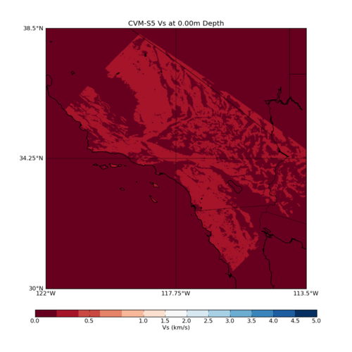
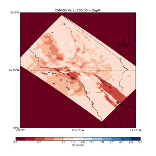
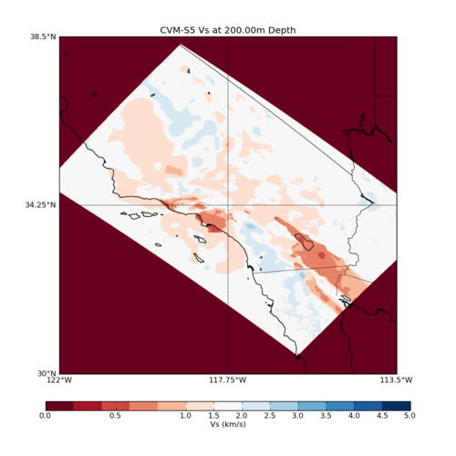
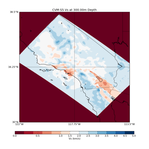
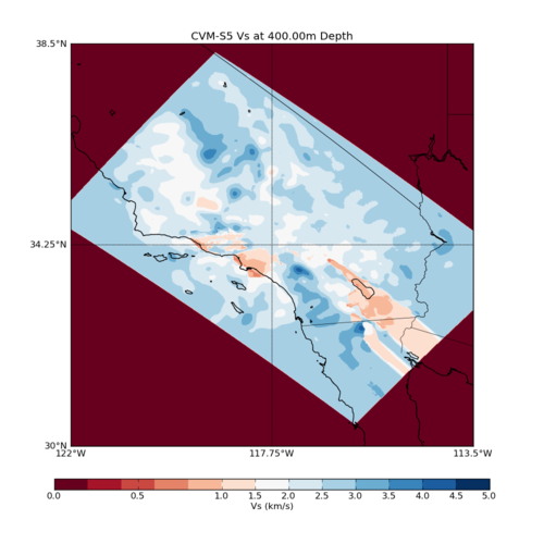
CVM-S5 is an improved version of the CVM-S4 velocity model which includes full 3D tomographic improvements to the SCEC 4 velocity model as well as an optional GTL implementation. Please note that unlike CVM-S4.26, CVM-S5 does not "merge" the results of the inversion with an underlying velocity model. Therefore it is strictly the 26th iteration dataset, 500m resolution, tri-linearly interpolated. There is no background model included, although UCVM can tile a background 1D model should the user specifically ask for it.
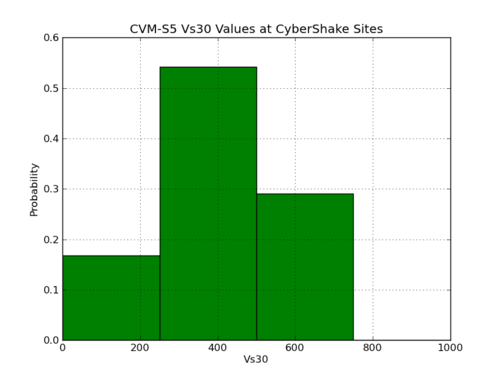
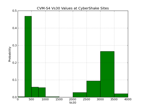
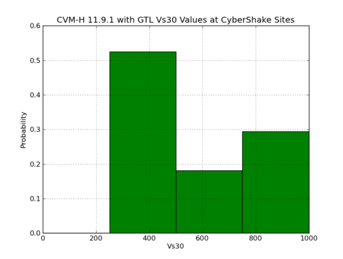
CyberShake Histogram Plots
Vs30 at CyberShake Sites
|
|
|
Z1.0 at CyberShake Sites
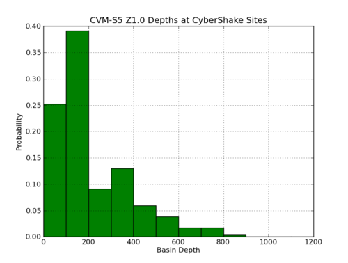
|
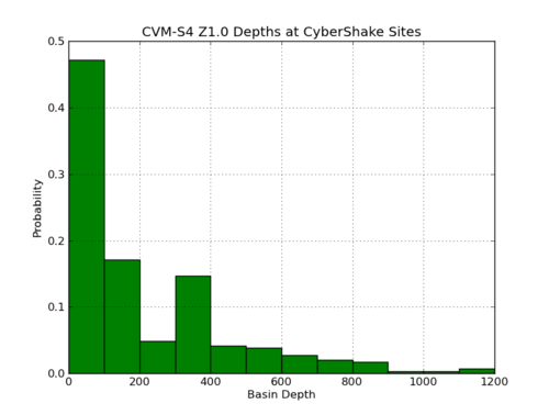
|
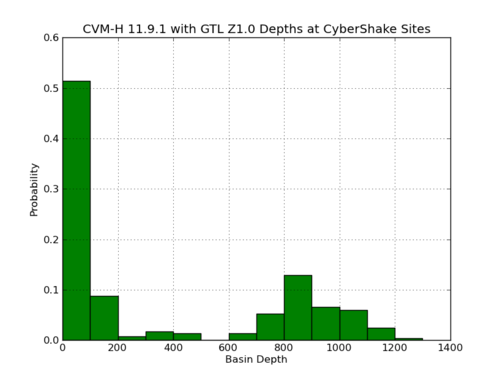
|
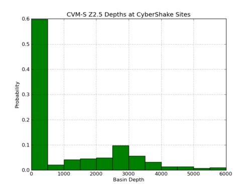
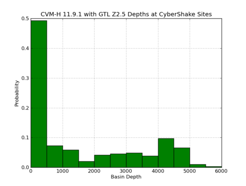
Z2.5 at CyberShake Sites
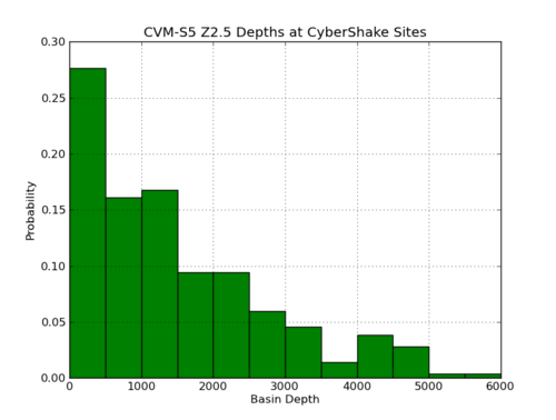
|
|
|
Material Properties Below 50km
The image below shows depth profiles for all CyberShake sites plotted onto one image. The depth goes from 0km to 500km.
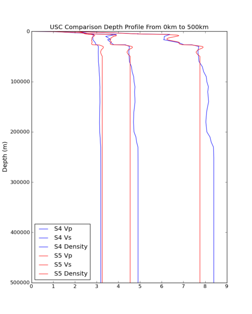
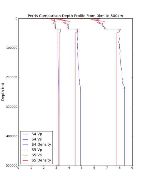
In the two images below, CVM-S5 is in red and CVM-S4 is in blue. Currently, CVM-S5 returns the material properties at 50km for all depths below 50km.
|
|
Attenuation Relationship
Attenuation is based off of Olsen et al., 2003 and is calculated as follows:
If Vs < 1500:
Qs = Vs * 0.02
Else:
Qs = Vs * 0.10
Qp = Qs * 1.5
Density Based on Vs
According to Po Chen:
"The Vs-density relation was obtained from Table 1 in Brocher 2005. In that table, the 3rd column is Vs and the 5th column is density. So I did a regression using data from these two columns and obtained a polynomial relation for Vs-density. Those numbers in that data file are the coefficients of the polynomial."
The actual polynomial is:
1.2948318548300342 + 1.2550758337054457Vs - 0.51231936640441489Vs2 + 0.051962399479341816Vs3 + 0.015600987888334450Vs4 - 0.0024189659303912917Vs5
Initial Plots
CVM-S5 0m to 500m with GTL
|
|
|
|
|

|
Depth Profiles
Surface Profiles
Del Amo -118.09624, 33.84822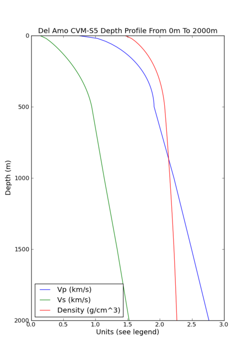
|
Diablo Canyon -120.85611, 35.21083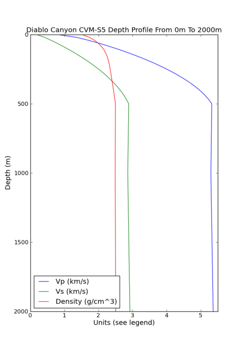
|
PERRIS -117.24904, 3380594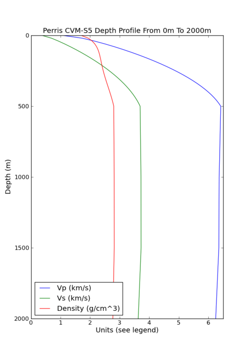
|
USC -118.286, 34.0192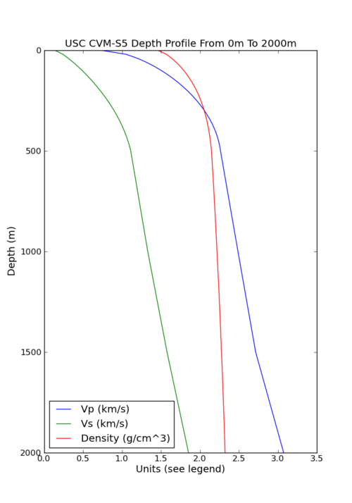
|
60km Profiles
Del Amo -118.09624, 33.84822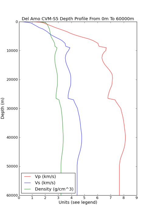
|
Diablo Canyon -120.85611, 35.21083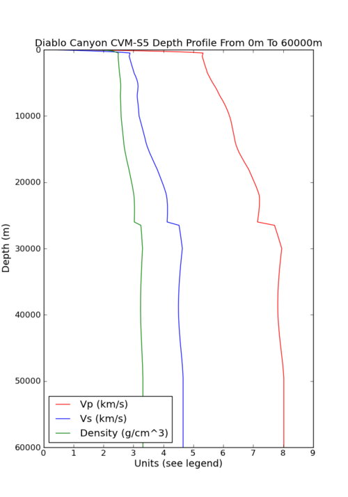
|
PERRIS -117.24904, 3380594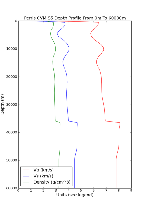
|
USC -118.286, 34.0192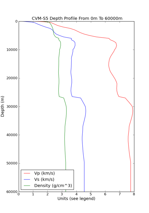
|
CVM-S5 0m to 500m no GTL
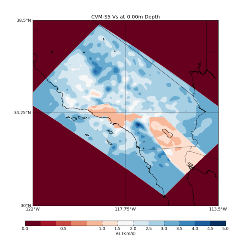
|

|
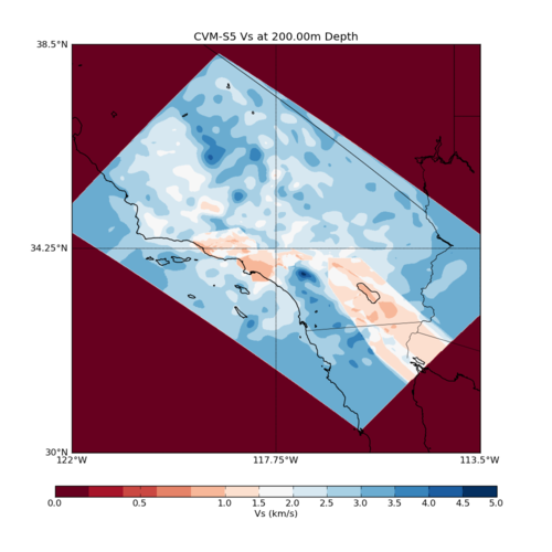
|

|

|
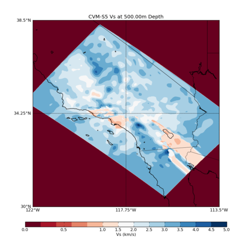
|
