Difference between revisions of "Hadley-Kanamori"
| Line 1: | Line 1: | ||
| + | Hadley Kanamori 1D model is used for various purposes in SCEC research, and by seismic networks in California. | ||
| + | |||
| + | == References == | ||
| + | A recent paper that cites the model and defines the layers. | ||
| + | #Hutton, K., Woessner, J., Hauksson, E. (2010) Earthquake Monitoring in Southern California for Seventy-Seven Years (1932-2008) BSSA, Vol. 100, No. 2, pp423-446, April 2010 | ||
| + | |||
| + | == Table == | ||
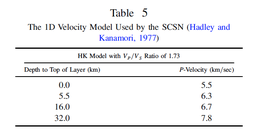
| + | [[Image:HadleyKanamori-1D.png|256px|thumb|left| Table 5 from Hutton et al 2010]] | ||
| + | |||
== SCSN HK == | == SCSN HK == | ||
| − | + | A text definition of the HK model is given below. SCSN uses a Vp/Vs ratio of 1.73 | |
| − | SCSN | ||
<pre> | <pre> | ||
| Line 12: | Line 20: | ||
== UCVM SCEC 1D Model Definition == | == UCVM SCEC 1D Model Definition == | ||
| + | SCEC uses a modified version of the HK model as a background model in their 3D velocity models. This means that if you query some of the Calfornia CVM's outside their defined coverage region, the CVM will return values from the HK model. In general, CVM tools will use linear interpolate between layers, so material properties returned vary gradually between model layers. | ||
<pre> | <pre> | ||
# 1D Velocity Model configuration | # 1D Velocity Model configuration | ||
| Line 36: | Line 45: | ||
== BBP Northridge/Whittier Narrows Model == | == BBP Northridge/Whittier Narrows Model == | ||
| + | SCEC provides an alternative LA Basin 1D model. This was defined by R. Graves using average Vp, Vs values for a number of sites in the LA Basin region. This model is often used as a 1D model for Los Angeles region ground motion simulations. | ||
| + | |||
<pre> | <pre> | ||
| − | |||
THICKNESS P-VEL S-VEL DENS QP QS | THICKNESS P-VEL S-VEL DENS QP QS | ||
0.0020 1.7000 0.4500 2.0000 45.0000 22.5000 | 0.0020 1.7000 0.4500 2.0000 45.0000 22.5000 | ||
| Line 57: | Line 67: | ||
10.0000 6.8000 3.8000 2.9500 380.0000 190.0000 | 10.0000 6.8000 3.8000 2.9500 380.0000 190.0000 | ||
999.0000 7.8000 4.5000 3.2000 450.0000 225.0000 | 999.0000 7.8000 4.5000 3.2000 450.0000 225.0000 | ||
| − | |||
</pre> | </pre> | ||
| Line 68: | Line 77: | ||
[[File:1d_bbp1d_linear.png|300px]] | [[File:1d_bbp1d_linear.png|300px]] | ||
| − | == | + | == Related Entries == |
| − | + | *[[UCVM]] | |
| − | + | *[CME_Project]] | |
| − | |||
| − | |||
Revision as of 21:28, 22 January 2017
Hadley Kanamori 1D model is used for various purposes in SCEC research, and by seismic networks in California.
Contents
References
A recent paper that cites the model and defines the layers.
- Hutton, K., Woessner, J., Hauksson, E. (2010) Earthquake Monitoring in Southern California for Seventy-Seven Years (1932-2008) BSSA, Vol. 100, No. 2, pp423-446, April 2010
Table
SCSN HK
A text definition of the HK model is given below. SCSN uses a Vp/Vs ratio of 1.73
Top of Layer (km)   P-Velocity (km/sec)
0.0          5.5
5.5          6.3
16.0        6.7
32.0        7.8
UCVM SCEC 1D Model Definition
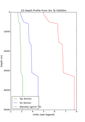
SCEC uses a modified version of the HK model as a background model in their 3D velocity models. This means that if you query some of the Calfornia CVM's outside their defined coverage region, the CVM will return values from the HK model. In general, CVM tools will use linear interpolate between layers, so material properties returned vary gradually between model layers.
# 1D Velocity Model configuration
#
# Vp is interpolated between layer n to n+1.
# Rho is derived from vp (./src/ucvm/ucvm_model_1d.c)
# Vs is derived from Vp and Rho (./src/ucvm/ucvm_model_1d.c)
#
version=Hadley-Kanamori 1D (CVM-S)

# Depth of model in layers
num_z=9

# Depth to start of layer (km)
depth_vals=1.0, 5.0, 6.0, 10.0, 15.5, 16.5, 22.0, 31.0, 33.0

# Vp at start of layer (km/s)
vp_vals=5.0, 5.5, 6.3, 6.3, 6.4, 6.7, 6.75, 6.8, 7.8
The model looks as follows:
BBP Northridge/Whittier Narrows Model
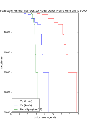
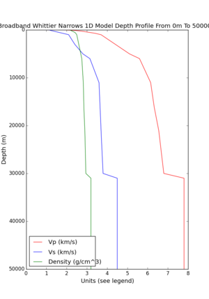
SCEC provides an alternative LA Basin 1D model. This was defined by R. Graves using average Vp, Vs values for a number of sites in the LA Basin region. This model is often used as a 1D model for Los Angeles region ground motion simulations.
THICKNESS	P-VEL	S-VEL	DENS	QP	QS
0.0020	1.7000	0.4500	2.0000	45.0000	22.5000
0.0040	1.8000	0.6500	2.1000	65.0000	32.5000
0.0060	1.8000	0.8500	2.1000	85.0000	42.5000
0.0080	1.9000	0.9500	2.1000	95.0000	47.5000
0.0100	2.0000	1.1500	2.2000	115.0000	57.5000
0.0700	2.4000	1.2000	2.2000	120.0000	60.0000
0.2000	2.8000	1.4000	2.3000	140.0000	70.0000
0.2000	3.1000	1.6000	2.4000	160.0000	80.0000
0.2000	3.4000	1.8000	2.4500	180.0000	90.0000
0.3000	3.7000	2.1000	2.5000	210.0000	105.0000
2.0000	4.4000	2.4000	2.6000	240.0000	120.0000
2.0000	5.1000	2.8000	2.7000	280.0000	140.0000
1.0000	5.6000	3.1500	2.7500	315.0000	157.5000
5.0000	6.1500	3.6000	2.8250	360.0000	180.0000
5.0000	6.3200	3.6500	2.8500	365.0000	182.5000
5.0000	6.5500	3.7000	2.9000	370.0000	185.0000
10.0000	6.8000	3.8000	2.9500	380.0000	190.0000
999.0000	7.8000	4.5000	3.2000	450.0000	225.0000
The non-interpolated (step) version of the model looks as follows:
The interpolated version of the model looks as follows:
Related Entries
- UCVM
- [CME_Project]]


