Difference between revisions of "CyberShake volume rotation"
| (54 intermediate revisions by the same user not shown) | |||
| Line 31: | Line 31: | ||
After running a series of tests, we identified that the difference seems to be related to the rotation angle: the smaller values are produced when running with a rotation angle of -55 degrees (what we have used in the past for southern California sites), and the larger values with a rotation of -30 degrees. Neither the site nor this source are near the volume boundaries. | After running a series of tests, we identified that the difference seems to be related to the rotation angle: the smaller values are produced when running with a rotation angle of -55 degrees (what we have used in the past for southern California sites), and the larger values with a rotation of -30 degrees. Neither the site nor this source are near the volume boundaries. | ||
| − | == 1D test == | + | == Study 18.8 vs Study 17.3 comparison == |
| + | |||
| + | Below are Rotd comparison plots for sites s845 and s835, hard rock sites which were included in both studies. | ||
| + | |||
| + | == 1D test, RWG == | ||
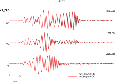
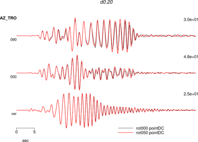
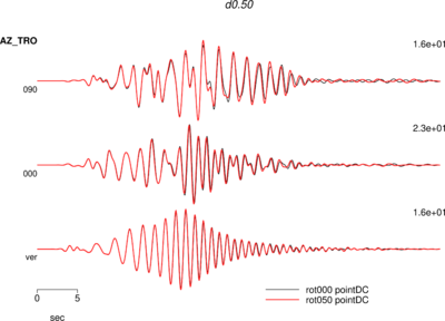
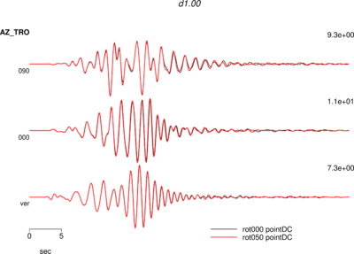
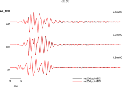
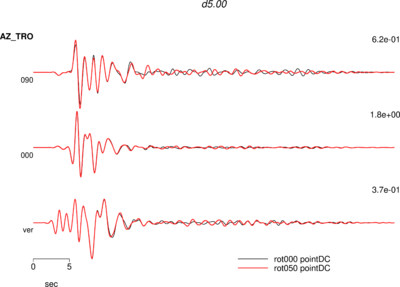
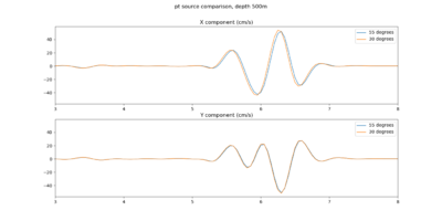
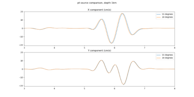
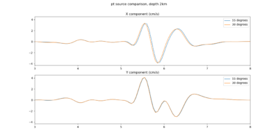
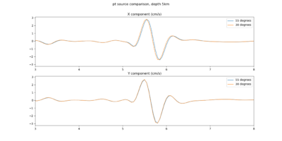
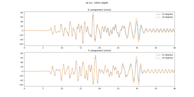
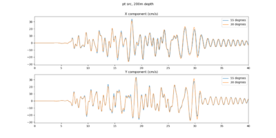
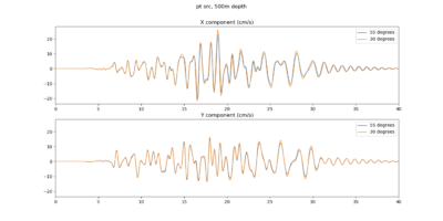
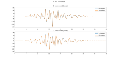
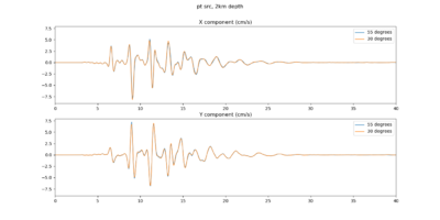
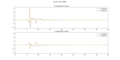
Rob Graves ran a 1D test in which seismograms were computed about 16 km from the source for rotation angles of 0 and -50 degrees. Below are plots comparing the three components at a variety of depths. | Rob Graves ran a 1D test in which seismograms were computed about 16 km from the source for rotation angles of 0 and -50 degrees. Below are plots comparing the three components at a variety of depths. | ||
| Line 40: | Line 44: | ||
|- | |- | ||
! 100m | ! 100m | ||
| − | | [[File:erf51_1D_RWG_SGT_test_d0.10.png|thumb| | + | | [[File:erf51_1D_RWG_SGT_test_d0.10.png|thumb|400px]] |
| + | |- | ||
| + | ! 200m | ||
| + | | [[File:erf51_1D_RWG_SGT_test_d0.20.png|thumb|400px]] | ||
| + | |- | ||
| + | ! 500m | ||
| + | | [[File:erf51_1D_RWG_SGT_test_d0.50.png|thumb|400px]] | ||
| + | |- | ||
| + | ! 1km | ||
| + | | [[File:erf51_1D_RWG_SGT_test_d1.00.png|thumb|400px]] | ||
| + | |- | ||
| + | ! 2km | ||
| + | | [[File:erf51_1D_RWG_SGT_test_d2.00.png|thumb|400px]] | ||
| + | |- | ||
| + | ! 5km | ||
| + | | [[File:erf51_1D_RWG_SGT_test_d5.00.png|thumb|400px]] | ||
| + | |} | ||
| + | |||
| + | == 1D test, AWP == | ||
| + | |||
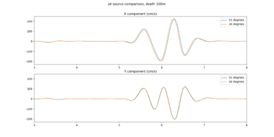
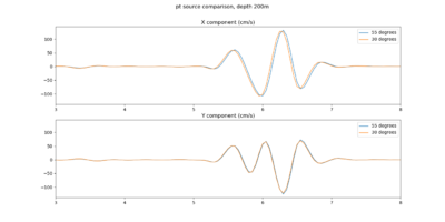
| + | We configured a similar test (point source, variety of depths, about 16 km from site) using the AWP SGT code and the Hadley-Kanamori 1D model. We see small differences with this code as well. | ||
| + | |||
| + | {| | ||
| + | ! depth | ||
| + | ! seismograms | ||
| + | |- | ||
| + | ! 100m | ||
| + | | [[File:erf51_1D_AWP_SGT_test_d0.10.png|thumb|400px]] | ||
| + | |- | ||
| + | ! 200m | ||
| + | | [[File:erf51_1D_AWP_SGT_test_d0.20.png|thumb|400px]] | ||
| + | |- | ||
| + | ! 500m | ||
| + | | [[File:erf51_1D_AWP_SGT_test_d0.50.png|thumb|400px]] | ||
| + | |- | ||
| + | ! 1km | ||
| + | | [[File:erf51_1D_AWP_SGT_test_d1.00.png|thumb|400px]] | ||
| + | |- | ||
| + | ! 2km | ||
| + | | [[File:erf51_1D_AWP_SGT_test_d2.00.png|thumb|400px]] | ||
| + | |- | ||
| + | ! 5km | ||
| + | | [[File:erf51_1D_AWP_SGT_test_d5.00.png|thumb|400px]] | ||
| + | |} | ||
| + | |||
| + | == 1D test, AWP, Mojave 1D model == | ||
| + | |||
| + | We repeated the above test using the BBP Mojave 1D model, the same model Rob used for his tests, and got much more similar results to Rob. | ||
| + | |||
| + | {| | ||
| + | ! depth | ||
| + | ! seismograms | ||
| + | |- | ||
| + | ! 100m | ||
| + | | [[File:erf51_1D_AWP_SGT_test_mojave_d0.10.png|thumb|400px]] | ||
|- | |- | ||
! 200m | ! 200m | ||
| − | | [[File: | + | | [[File:erf51_1D_AWP_SGT_test_mojave_d0.20.png|thumb|400px]] |
|- | |- | ||
! 500m | ! 500m | ||
| − | | [[File: | + | | [[File:erf51_1D_AWP_SGT_test_mojave_d0.50.png|thumb|400px]] |
|- | |- | ||
! 1km | ! 1km | ||
| − | | [[File: | + | | [[File:erf51_1D_AWP_SGT_test_mojave_d1.00.png|thumb|400px]] |
|- | |- | ||
! 2km | ! 2km | ||
| − | | [[File: | + | | [[File:erf51_1D_AWP_SGT_test_mojave_d2.00.png|thumb|400px]] |
|- | |- | ||
! 5km | ! 5km | ||
| − | | [[File: | + | | [[File:erf51_1D_AWP_SGT_test_mojave_d5.00.png|thumb|400px]] |
| + | |} | ||
| + | |||
| + | == ERF 36 (UCERF2, 200m spacing) test == | ||
| + | |||
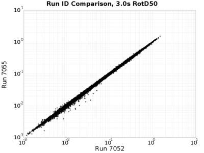
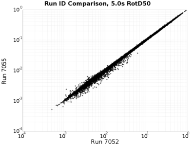
| + | We ran site USC using CVM-S4.26.M01 with -30 degree rotation, and compared the results to the 'standard' Southern California rotation of -55 degrees. | ||
| + | |||
| + | Overall, the differences get smaller as the ground motions get larger, and the hazard curves are visually identical, suggesting that the rotation angle has a negligible effect on hazard for UCERF2 simulations. | ||
| + | |||
| + | {| | ||
| + | ! !! 3 sec !! 5 sec !! 10 sec | ||
| + | |- | ||
| + | ! RotD comparisons | ||
| + | | [[File:erf36_7052_v_7055_rotd_comparison_3sec.png|thumb|400px]] | ||
| + | | [[File:erf36_7052_v_7055_rotd_comparison_5sec.png|thumb|400px]] | ||
| + | | [[File:erf36_7052_v_7055_rotd_comparison_10sec.png|thumb|400px]] | ||
| + | |- | ||
| + | ! Hazard curves | ||
| + | | [[File:erf36_7052_v_7055_comparison_3sec.png|thumb|400px]] | ||
| + | | [[File:erf36_7052_v_7055_comparison_5sec.png|thumb|400px]] | ||
| + | | [[File:erf36_7052_v_7055_comparison_10sec.png|thumb|400px]] | ||
| + | |} | ||
| + | |||
| + | Note that the dropoff off the black curve in the 3 sec plot after 1 g is due to the fact that the black and blue curves are sampled at different X-values. | ||
| + | |||
| + | == ERF 36 1D test == | ||
| + | |||
| + | We repeated the above test, but using the UCVM built-in SCEC 1D velocity model. These results show slightly less scatter than the 3D results, but it's more asymmetric. | ||
| + | Note that run 7056 (the X-axis) was done with a volume rotated -55 degrees, and 7057 with -30 degrees. | ||
| + | |||
| + | {| | ||
| + | ! !! 3 sec !! 5 sec !! 10 sec | ||
| + | |- | ||
| + | ! RotD comparisons | ||
| + | | [[File:erf36_7056_v_7057_rotd_comparison_3sec.png|thumb|400px]] | ||
| + | | [[File:erf36_7056_v_7057_rotd_comparison_5sec.png|thumb|400px]] | ||
| + | | [[File:erf36_7056_v_7057_rotd_comparison_10sec.png|thumb|400px]] | ||
| + | |} | ||
| + | |||
| + | Here are statistics on the above runs: | ||
| + | |||
| + | {| border="1" cellpadding="2" | ||
| + | ! !! Differences (run 7057 - run 7056)<br>of linear values (cm/s2) !! Differences of natural log values !! Linear Ratios (run 7057/run 7056) | ||
| + | |- | ||
| + | ! Min | ||
| + | | -12.929062 || -0.170983 || 0.842836 | ||
| + | |- | ||
| + | ! Max | ||
| + | | 12.866089 || 0.591074 || 1.805926 | ||
| + | |- | ||
| + | ! Mean | ||
| + | | 0.031936 || 0.001222 || 1.001283 | ||
| + | |- | ||
| + | ! Std Dev | ||
| + | | 0.363081 || 0.010961 || 0.011117 | ||
| + | |- | ||
| + | ! Mean Abs | ||
| + | | 0.193350 || 0.007560 | ||
| + | |} | ||
| + | |||
| + | We also created plots comparing the difference and ratios to shortest site-rupture distance and magnitude. | ||
| + | |||
| + | {| | ||
| + | ! !! Difference (cm/s2) !! Ratio | ||
| + | |- | ||
| + | ! Magnitude | ||
| + | | [[File:7056_v_7057_diff_mag_3sec.png|thumb|400px]] | ||
| + | | [[File:7056_v_7057_ratio_mag_3sec.png|thumb|400px]] | ||
| + | |- | ||
| + | ! Distance | ||
| + | | [[File:7056_v_7057_diff_dist_3sec.png|thumb|400px]] | ||
| + | | [[File:7056_v_7057_ratio_dist_3sec.png|thumb|400px]] | ||
| + | |} | ||
| + | |||
| + | == ERF 36 Mojave 1D test == | ||
| + | |||
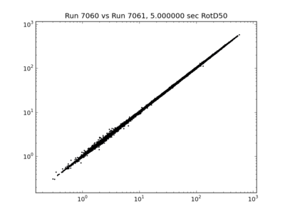
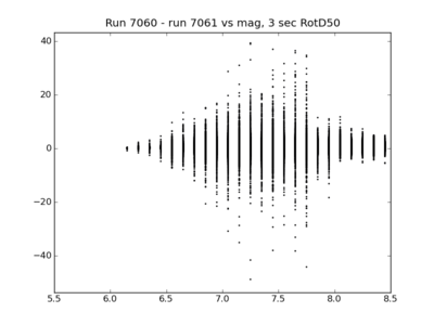
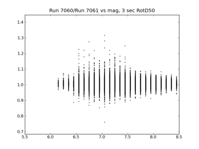
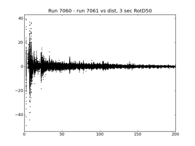
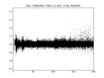
| + | We repeated the above test again, but this time using the Mojave 1D model from the BBP, which has much lower near-surface velocities than the Hadley-Kanamori 1D model. Run 7060 was done with -30 degrees, and run 7061 with -55 degrees. | ||
| + | |||
| + | {| | ||
| + | ! !! 3 sec !! 5 sec !! 10 sec | ||
| + | |- | ||
| + | ! RotD comparisons | ||
| + | | [[File:7060_v_7061_rotd_comparison_3sec.png|thumb|400px]] | ||
| + | | [[File:7060_v_7061_rotd_comparison_5sec.png|thumb|400px]] | ||
| + | | [[File:7060_v_7061_rotd_comparison_10sec.png|thumb|400px]] | ||
| + | |} | ||
| + | |||
| + | Here are statistics on the above runs, for 3 sec RotD50: | ||
| + | |||
| + | {| border="1" cellpadding="2" | ||
| + | ! !! Differences (run 7060 - run 7061)<br>of linear values (cm/s2) !! Differences of natural log values !! Linear Ratios (run 7060/run 7061) | ||
| + | |- | ||
| + | ! Min | ||
| + | | -48.872131 || -0.27381 || 0.760476 | ||
| + | |- | ||
| + | ! Max | ||
| + | | 39.215027 || 0.273622 ||1.314718 | ||
| + | |- | ||
| + | ! Mean | ||
| + | | 0.223698 || 0.004606 || 1.004685 | ||
| + | |- | ||
| + | ! Std Dev | ||
| + | | 1.021811 || 0.011675 || 0.011753 | ||
| + | |- | ||
| + | ! Mean Abs | ||
| + | | 0.483368 || 0.009155 | ||
| + | |} | ||
| + | |||
| + | Here are plots comparing the difference and ratios to shortest site-rupture distance and magnitude at 3 sec. | ||
| + | |||
| + | {| | ||
| + | ! !! Difference (cm/s2) !! Ratio | ||
| + | |- | ||
| + | ! Magnitude | ||
| + | | [[File:7060_v_7061_diff_mag_3sec.png|thumb|400px]] | ||
| + | | [[File:7060_v_7061_ratio_mag_3sec.png|thumb|400px]] | ||
| + | |- | ||
| + | ! Distance | ||
| + | | [[File:7060_v_7061_diff_dist_3sec.png|thumb|400px]] | ||
| + | | [[File:7060_v_7061_ratio_dist_3sec.png|thumb|400px]] | ||
| + | |} | ||
| + | |||
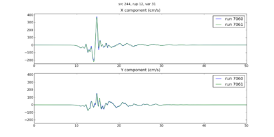
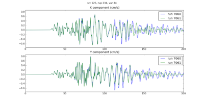
| + | We extracted seismograms for the biggest difference at 3 sec (48.9 cm/s2, for source 244, rupture 12, rup var 31) and biggest ratio (1.3, for source 125, rupture 234, rup var 34), below. The Garlock fault is about 50 km from the 30 degree volume boundary, and about 40 km from the 55 degree volume boundary, so the late differences in the Garlock seismograms may be due to boundary effects. However, the amplitude of these waves is very small - less than 1 cm/s. | ||
| + | |||
| + | {| | ||
| + | ! Biggest difference (M7.25 Puente Hills) !! Biggest ratio (M7.05 Garlock) | ||
| + | |- | ||
| + | | [[File:7060_v_7061_s244_r12_v31.png|thumb|400px]] | ||
| + | | [[File:7060_v_7061_s125_r234_v34.png|thumb|400px]] | ||
|} | |} | ||
| + | |||
| + | === Boundary effects === | ||
| + | |||
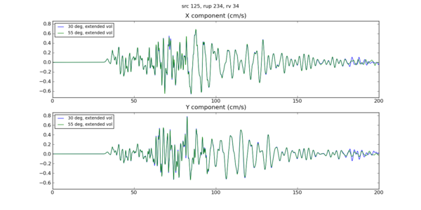
| + | To test the theory that the difference we see in the Garlock seismograms is due to boundary effects, we recalculated results for the above Garlock event, but with volumes which extended an extra ~100km to the northeast, moving the fault more than 140 km away from a boundary. | ||
| + | |||
| + | The two seismograms with different angles show much better agreement when not near the boundary. | ||
| + | |||
| + | {| | ||
| + | | [[File:s125_r234_v34_ext_vol_compare.png|thumb|600px]] | ||
| + | |} | ||
| + | |||
| + | When compared to the seismograms near the boundary with the normal-sized volume, these new results are different from both: | ||
| + | |||
| + | {| | ||
| + | | [[File:s125_r234_v34_vol_rot_compare.png|thumb|600px]] | ||
| + | |} | ||
| + | |||
| + | === Sponge zone tests === | ||
| + | |||
| + | We realized the sponge zone widths were only 20 points, so we tried rerunning with different values. | ||
| + | |||
| + | With 50 and 80 points, we still see differences in the seismograms from the ones 100km+ from the volume boundary: | ||
| + | |||
| + | {| | ||
| + | | [[File:sponge_zone_30deg_s125_r234_v34_compare.png|thumb|600px]] | ||
| + | |- | ||
| + | | [[File:sponge_zone_s125_r234_v34_compare.png|thumb|600px]] | ||
| + | |} | ||
| + | |||
| + | Here's a comparison of the RotD spectral plots for the 30 deg rotation, for various sponge values: | ||
| + | |||
| + | {| | ||
| + | | [[File:sponge_zone_30deg_rotd_s125_r234_v34_compare.png|thumb|600px]] | ||
| + | |} | ||
| + | |||
| + | Since there is no clear winner, we have decided to move ahead with '''50 points''' as a balance between reducing reflections and losing energy. | ||
Latest revision as of 20:18, 10 February 2020
This page documents the differences we see in results when using volumes with different rotation angles, and the investigation of these differences.
Contents
Problem description
When attempting to replicate on Summit results for site USC using ERF 51 (an RSQSim-based ERF) originally obtained on Blue Waters, we ran into some difficulty.
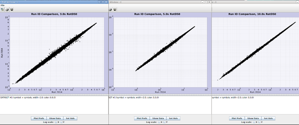
The plot below shows a comparison of RotD values obtained on Summit (Run ID 7054) vs on Blue Waters (Run ID 7014). As you can see, there is a general trend but more scatter than anticipated; the two results should match almost exactly.
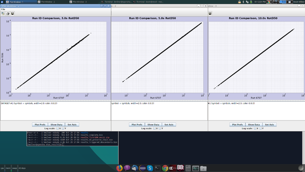
As a point of comparison, here are the same plots for the USC ERF 36 verification runs:
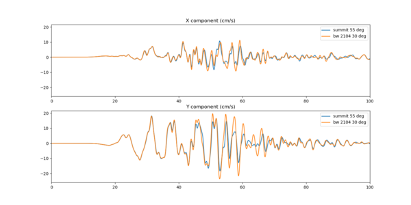
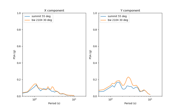
In particular, we identified source 684, rupture 323 as an event to investigate further. At a frequency of 3 seconds, the values obtained on Blue Waters were almost twice as big as those on Summit, 0.23 cm/s2 vs 0.12 cm/s2.
Below are plots comparing the seismograms and the geometric mean PSA values for these events on the two systems. The seismograms start to diverge after about 45 sec, and the geometric mean PSA values show the largest difference at about 3 sec.
Rotation angle
After running a series of tests, we identified that the difference seems to be related to the rotation angle: the smaller values are produced when running with a rotation angle of -55 degrees (what we have used in the past for southern California sites), and the larger values with a rotation of -30 degrees. Neither the site nor this source are near the volume boundaries.
Study 18.8 vs Study 17.3 comparison
Below are Rotd comparison plots for sites s845 and s835, hard rock sites which were included in both studies.
1D test, RWG
Rob Graves ran a 1D test in which seismograms were computed about 16 km from the source for rotation angles of 0 and -50 degrees. Below are plots comparing the three components at a variety of depths.
| depth | seismograms |
|---|---|
| 100m | |
| 200m | |
| 500m | |
| 1km | |
| 2km | |
| 5km |
1D test, AWP
We configured a similar test (point source, variety of depths, about 16 km from site) using the AWP SGT code and the Hadley-Kanamori 1D model. We see small differences with this code as well.
| depth | seismograms |
|---|---|
| 100m | |
| 200m | |
| 500m | |
| 1km | |
| 2km | |
| 5km |
1D test, AWP, Mojave 1D model
We repeated the above test using the BBP Mojave 1D model, the same model Rob used for his tests, and got much more similar results to Rob.
| depth | seismograms |
|---|---|
| 100m | |
| 200m | |
| 500m | |
| 1km | |
| 2km | |
| 5km |
ERF 36 (UCERF2, 200m spacing) test
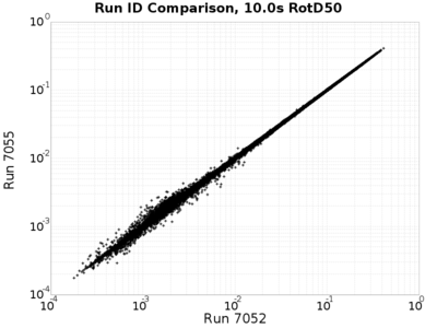
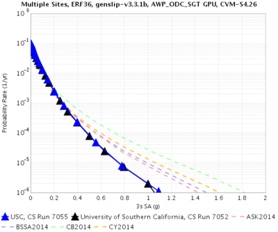
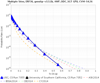
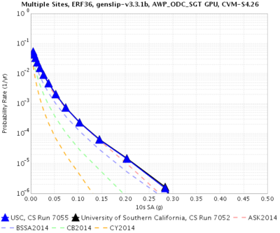
We ran site USC using CVM-S4.26.M01 with -30 degree rotation, and compared the results to the 'standard' Southern California rotation of -55 degrees.
Overall, the differences get smaller as the ground motions get larger, and the hazard curves are visually identical, suggesting that the rotation angle has a negligible effect on hazard for UCERF2 simulations.
| 3 sec | 5 sec | 10 sec | |
|---|---|---|---|
| RotD comparisons | |||
| Hazard curves |
Note that the dropoff off the black curve in the 3 sec plot after 1 g is due to the fact that the black and blue curves are sampled at different X-values.
ERF 36 1D test
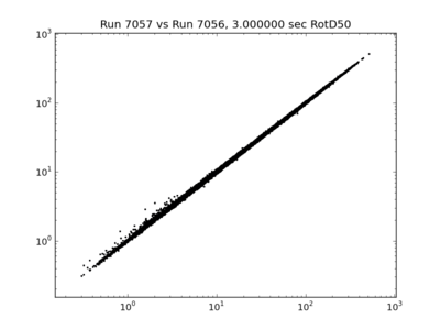
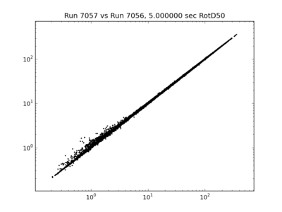
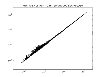
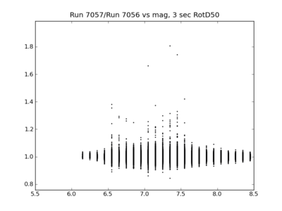
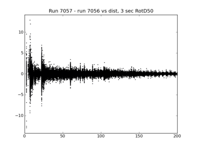
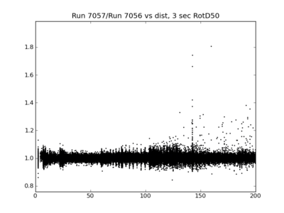
We repeated the above test, but using the UCVM built-in SCEC 1D velocity model. These results show slightly less scatter than the 3D results, but it's more asymmetric. Note that run 7056 (the X-axis) was done with a volume rotated -55 degrees, and 7057 with -30 degrees.
| 3 sec | 5 sec | 10 sec | |
|---|---|---|---|
| RotD comparisons |
Here are statistics on the above runs:
| Differences (run 7057 - run 7056) of linear values (cm/s2) |
Differences of natural log values | Linear Ratios (run 7057/run 7056) | |
|---|---|---|---|
| Min | -12.929062 | -0.170983 | 0.842836 |
| Max | 12.866089 | 0.591074 | 1.805926 |
| Mean | 0.031936 | 0.001222 | 1.001283 |
| Std Dev | 0.363081 | 0.010961 | 0.011117 |
| Mean Abs | 0.193350 | 0.007560 |
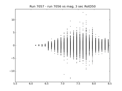
We also created plots comparing the difference and ratios to shortest site-rupture distance and magnitude.
| Difference (cm/s2) | Ratio | |
|---|---|---|
| Magnitude | ||
| Distance |
ERF 36 Mojave 1D test
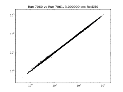
We repeated the above test again, but this time using the Mojave 1D model from the BBP, which has much lower near-surface velocities than the Hadley-Kanamori 1D model. Run 7060 was done with -30 degrees, and run 7061 with -55 degrees.
| 3 sec | 5 sec | 10 sec | |
|---|---|---|---|
| RotD comparisons |
Here are statistics on the above runs, for 3 sec RotD50:
| Differences (run 7060 - run 7061) of linear values (cm/s2) |
Differences of natural log values | Linear Ratios (run 7060/run 7061) | |
|---|---|---|---|
| Min | -48.872131 | -0.27381 | 0.760476 |
| Max | 39.215027 | 0.273622 | 1.314718 |
| Mean | 0.223698 | 0.004606 | 1.004685 |
| Std Dev | 1.021811 | 0.011675 | 0.011753 |
| Mean Abs | 0.483368 | 0.009155 |
Here are plots comparing the difference and ratios to shortest site-rupture distance and magnitude at 3 sec.
| Difference (cm/s2) | Ratio | |
|---|---|---|
| Magnitude | ||
| Distance |
We extracted seismograms for the biggest difference at 3 sec (48.9 cm/s2, for source 244, rupture 12, rup var 31) and biggest ratio (1.3, for source 125, rupture 234, rup var 34), below. The Garlock fault is about 50 km from the 30 degree volume boundary, and about 40 km from the 55 degree volume boundary, so the late differences in the Garlock seismograms may be due to boundary effects. However, the amplitude of these waves is very small - less than 1 cm/s.
| Biggest difference (M7.25 Puente Hills) | Biggest ratio (M7.05 Garlock) |
|---|---|
Boundary effects
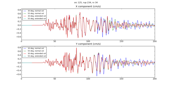
To test the theory that the difference we see in the Garlock seismograms is due to boundary effects, we recalculated results for the above Garlock event, but with volumes which extended an extra ~100km to the northeast, moving the fault more than 140 km away from a boundary.
The two seismograms with different angles show much better agreement when not near the boundary.
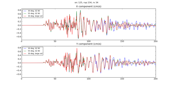
When compared to the seismograms near the boundary with the normal-sized volume, these new results are different from both:
Sponge zone tests
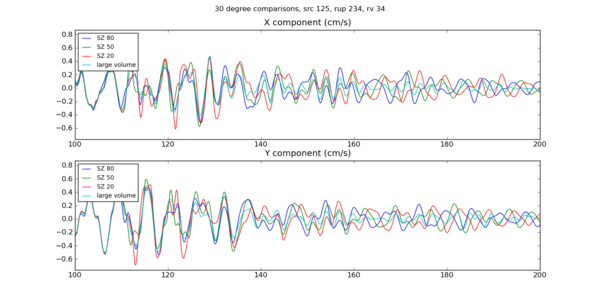
We realized the sponge zone widths were only 20 points, so we tried rerunning with different values.
With 50 and 80 points, we still see differences in the seismograms from the ones 100km+ from the volume boundary:
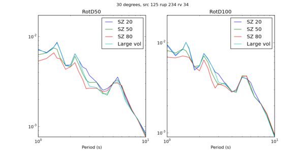
Here's a comparison of the RotD spectral plots for the 30 deg rotation, for various sponge values:
Since there is no clear winner, we have decided to move ahead with 50 points as a balance between reducing reflections and losing energy.
