CyberShake Study 21.12

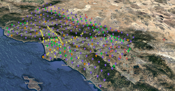
CyberShake 21.12 is a computational study to use a new ERF with CyberShake, generated from an RSQSim catalog. We plan to calculate results for 335 sites in Southern California using the RSQSim ERF, a minimum Vs of 500 m/s, and a frequency of 1 Hz. We will use the CVM-S4.26.M01 model, and the GPU implementation of AWP-ODC-SGT enhanced from the BBP verification testing. We will begin by generating all sets of SGTs, on Summit, then post-process them on a combination of Summit and Frontera.

Status

This study is in the pre-production phase. Production is scheduled to begin in mid-December, 2021.

Science Goals

The science goals for this study are:

• Calculate a regional CyberShake model using an alternative, RSQSim-derived ERF.
• Compare results from an RSQSim ERF to results using a UCERF2 ERF (Study 15.4).
• Quantify effects of source model non-ergodicity
• Compare spatial distribution of ground motions (including directivity) to empirical and kinematic models

Technical Goals

The technical goals for this study are:

• Perform a study using OLCF Summit as a key compute resource.
• Evaluate the performance of the new workflow submission host, shock-carc.
• Use Globus Online for staging of output data products.

ERF

The ERF was generated from an RSQSim catalog, with the following parameters:

• 715kyr catalog (the first 65k years of events were dropped, so that every fault's first event is excluded)
• 220,927 earthquakes with M6.5+
• All events have equal probability, 1/715k

Additional details are available on the catalog's metadata page, and the catalog and input fault geometry files can be downloaded from zeonodo. This is the catalog used in Milner et al., 2021, which used 0.5 Hz CyberShake simulations performed in May, 2020.

Sites

We will run a list of 335 sites, taken from the site list that was used in other Southern California studies. The order of execution will be:

• 10 sites used in Milner et al. (2021), each with top mesh point Vs at the 500 m/s floor: USC, SMCA, OSI, WSS, SBSM, LAF, s022, STNI, WNGC, PDE
• PAS hard rock site
• 20 km site grid
• 10 km site grid
• Remaining POIs, select 5km grid sites also used in Study 15.4

• CSV site list
• KML site list with names
• KML site list without names

Velocity Model

We will use CVM-S4.26.M01.

To better represent the near-surface layer, we will populate the velocity parameters for the surface point by querying the velocity model at a depth of (grid spacing)/4. For this study, the grid spacing is 100m, so we will query UCVM at a depth of 25m and use that value to populate the surface grid point. The rationale is that the media parameters at the surface grid point are supposed to represent the material properties for [0, 50m], and this is better represented by using the value at 25m than the value at 0m.

Verification Tests

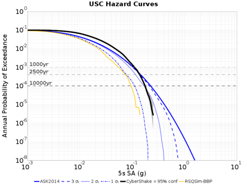
USC Hazard Curves

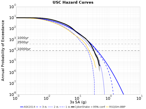
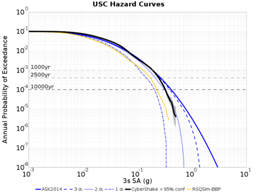
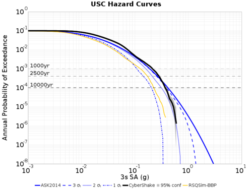
Hazard curve comparisons for site USC, between:

• ERF 58: 0.5 Hz RSQSim ERF used for Milner et al. (2021) calculations, May 2020
• ERF 61: 0.5 Hz RSQSim production ERF with the same catalog
• ERF 62: 1 Hz RSQSim production ERF with the same catalog

The first test run of ERF 61 used the wrong (older) mesh lower depth of 40 km, which is why the top right plot differs slightly from the top left. The bottom left plot agrees perfectly with the tol left.

ERF 58, Original	ERF 61 w/ wrong depth
ERF 61 w/ corrected depth	ERF 62 (1 Hz) with old simulation parameters

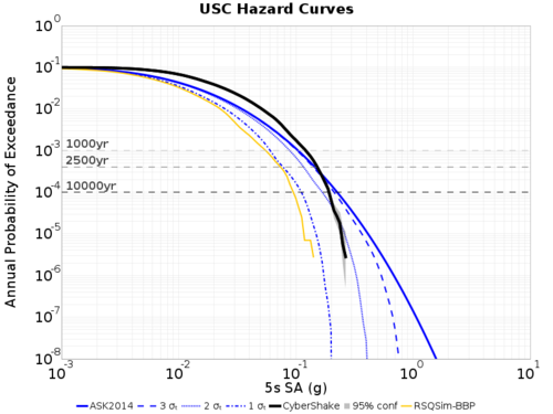
The first 1 Hz test run uses (bottom right above) uses the same simulation paramters as used with ERF 58 and 61, changing only the frequency. Some differences are apparent, which also persist for longer period (5s) curves:

ERF 61, 5s Sa, 0.5 Hz, old simulation parameters	ERF 62, 5s Sa, 1 Hz, old simulation parameters

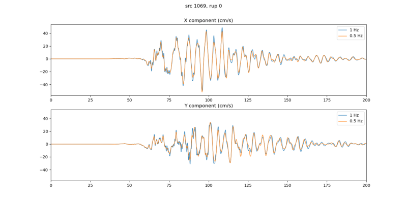
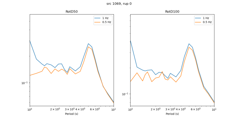
Here are seismograms and RotD's for the largest amplitude rupture for this 0.5 Hz vs 1 Hz test:

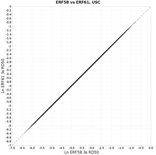
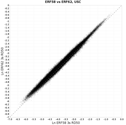
3s Amplitude Scatter plots

These plots show that (left) ERF 61 exactly reproduces ERF 58, and (right) that there are indeed differences going from 0.5 Hz to 1 Hz:

Technical and Scientific Updates

Since our last study we have made a number of scientific updates to the platform, many as a result of the BBP verification effort.

• Several bugs were found and fixed in the AWP code.
• We have switched from stress insertion to velocity insertion of the impulse when generating SGTs.
• The sponge zone used in the absorbing boundary condition was increased from 50 to 80 points.
• By default, we use a depth of h/4 when querying UCVM to populate the surface grid point.
• The padding between the nearest fault or site and the edge of the volume was increased from 30 to 50 km.
• We fixed a bug in the coordinate conversion between RWG and AWP: previously we were adding 1 to the RWG z-coordinate to produce the AWP z-coordinate, but both codes use z=1 to represent the surface and therefore no increment should be applied.
• When calculating Qs in the SGT header generation code, a default Qs of 25 was always used. This has been changed to Qs=0.05Vs.
• We have turned off the adjustment of mu and lambda.
• FP was increased from 0.5 to 1.0.
• We modified the lambda and mu calculations in AWP to use the original media parameter values from the velocity mesh rather than the FP-modified ones when calculating strains, to be consistent with RWG.

Study 18.8 Lessons Learned

• Consider separating SGT and PP workflows in auto-submit tool to better manage the number of each, for improved reservation utilization.
• Create a read-only way to look at the CyberShake Run Manager website.
• Consider reducing levels of the workflow hierarchy, thereby reducing load on shock.
• Determine advance plan for SGTs for sites which require fewer GPUs.
• Determine advance plan for SGTs for sites which exceed memory on nodes.
• Create new velocity model ID for composite model, capturing metadata.

We modified the database to enable composite models, but for this study we are just using a single model.

• Verify all Java processes grab a reasonable amount of memory.
• Clear disk space before study begins to avoid disk contention.
• Add stress test before beginning study, for multiple sites at a time, with cleanup.
• In addition to disk space, check local inode usage.

Only 1% of the inodes are used on shock-carc; we will assume /project has sufficient inodes, as we can't check them.

• Establish clear rules and policies about reservation usage.
• If submitting to multiple reservations, make sure enough jobs are eligible to run that no reservation is starved.

We are not planning to run this study with reservations.

• If running primarily SGTs for awhile, make sure they don't get deleted due to quota policies.

We will stage the SGTs to HPSS if there is a delay in post-processing them. Summit has a 90-day purge policy, so we will have some time.

Output Data Products

File-based data products

We plan to produce the following data products which will be stored at CARC:

• Seismograms: 2-component seismograms, 8000 timesteps (400 sec) each
• PSA: X and Y spectral acceleration at 44 periods (10, 9.5, 9, 8.5, 8, 7.5, 7, 6.5, 6, 5.5, 5, 4.8, 4.6, 4.4, 4.2, 4, 3.8, 3.6, 3.4, 3.2, 3, 2.8, 2.6, 2.4, 2.2, 2, 1.66667, 1.42857, 1.25, 1.11111, 1, .66667, .5, .4, .33333, .285714, .25, .22222, .2, .16667, .142857, .125, .11111, .1 sec)
• RotD: RotD50, the RotD50 azimuth, and RotD100 at 22 periods (1.0, 1.2, 1.4, 1.5, 1.6, 1.8, 2.0, 2.2, 2.4, 2.6, 2.8, 3.0, 3.5, 4.0, 4.4, 5.0, 5.5, 6.0, 6.5, 7.5, 8.5, 10.0 sec)
• Durations: for X and Y components, energy integral, Arias intensity, cumulative absolute velocity (CAV), and for both velocity and acceleration, 5-75%, 5-95%, and 20-80%.

Database data products

We plan to store the following data products in the database:

• PSA: none
• RotD: RotD50 and RotD100 at 10, 7.5, 5, 4, 3, and 2 sec.
• Durations: acceleration 5-75% and 5-95% for X and Y components

Computational and Data Estimates

Computational Estimates

We based these estimates by scaling from site USC (the average site has 3.8% more events and a volume 9.7% larger).

SGT calculation

	UCVM runtime	UCVM nodes	SGT runtime	SGT nodes	Other SGT workflow jobs	Summit Total
USC	372 sec	80	2628 sec	67	1510 node-sec	106.5 node-hrs
Average (est)	408 sec	80	2883 sec	67	1550 node-sec	116.8 node-hrs

Adding 10% overrun margin gives us an estimate of 43k node-hours for SGT calculation.

PP calculation

	DirectSynth runtime	DirectSynth nodes	Summit Total
USC	1081	36	10.8
Average (est)	1122	36	11.2

Adding 10% overrun margin gives an estimate of 4.2k node-hours for post-processing.

Data Estimates

Summit

Data estimates

	Velocity mesh	SGTs size	Temp data	Output data
USC	243 GB	196 GB	439 GB	4.5 GB
Average	267 GB	203 GB	470 GB	4.7 GB
Total	87 TB	66 TB	153 TB	1.5 TB

This is a total of 307 TB, which we could reach if we calculate all the SGTs first and don't delete anything. The default quota on Summit is 50 TB, so I suggest we request a quota increase to at least 300 TB so we don't need to rely on cleanup.

If we need to keep the SGTs for awhile before performing post-processing, the quota on HPSS is 100 TB, so we could store them there.

CARC

We estimate 1.5 TB in output data, which will be transferred back to CARC.

shock-carc

The study should use approximately 200 GB in workflow log space on /home/shock. This drive has approximately 1.7 TB free.

moment database

The PeakAmplitudes table uses approximately 100 bytes per entry.

100 bytes/entry * 16 entries/event * 76786 events/site * 335 sites = 38 GB. The drive on moment with the mysql database has 919 GB free.

Production Checklist

Science:

• Confirm that ERF 62 test produces results which closely match ERF 61
• Restore improvements to codes since ERF 58, and rerun USC for ERF 62
• Fix h/4 issue and rerun USC test.
• Create prioritized site list.
• Hold science readiness review.
• Add link to fault geometry on Zenodo, either on the wiki or the fault metadata page.
• Add copy of science readiness review slides to wiki.
• Generate 0.5 Hz v 1 Hz scatterplot from UCERF2 ERF run.
• Go through config updates as a pair to confirm they have been correctly applied.

Technical:

• Approach OLCF for the following requests:
  • Quota increase to 400 TB
  • 8 jobs ready to run
  • 5 jobs in bin 5.
• To be able to bundle jobs, fix issue with Summit glideins.
• To run post-processing, resolve issues using GO to transfer data back to /project at CARC.
• Tag code
• Modify job sizes and runtimes.
• Test auto-submit script.
• Prepare pending file.
• Create XML file describing study for web monitoring tool.
• Get usage stats for Summit.
• Prepare cronjob on Summit for monitoring jobs.
• Call with OLCF staff
• Activate script for monitoring x509 certificate.
• Modify workflows to not insert or calculate curves for PSA data.
• Modify dax-generator to use h/4 as default for surface point.
• Modify dax-generator to use ERF62 parameter file for generating GMPE comparison curves.
• Hold technical readiness review.
• Modify nt to 8000 (400 sec).
• Add calculation of PGV.
• Test SGT-only and PP-only create/plan/run scripts.