Difference between revisions of "CyberShake BBP Verification"
(→Events) |
|||
| (32 intermediate revisions by the same user not shown) | |||
| Line 1: | Line 1: | ||
| − | This page documents our CyberShake Broadband Platform | + | This page documents our initial CyberShake Broadband Platform verification work, running the BBP validation events through CyberShake. |
== Events == | == Events == | ||
| − | We plan to run the | + | The BBP has support for the following events. We plan to run the ones in bold: |
| − | + | <ul> | |
| − | * | + | <li>Alum Rock Mw 5.45</li> |
| − | + | <li><b>Chino Hills Mw 5.39</b></li> | |
| − | + | <li><b>Hector Mine Mw 7.13</b></li> | |
| − | * | + | <li><b>Landers Mw Mw 7.22*</b></li> |
| − | * | + | <li>Loma Prieta Mw 6.94</li> |
| + | <li><b>North Palm Springs Mw 6.12</b></li> | ||
| + | <li><b>Northridge Mw 6.73</b></li> | ||
| + | <li>Parkfield Mw 6.0</li> | ||
| + | <li><b>Ridgecrest A Mw 6.47</b></li> | ||
| + | <li>Ridgecrest B Mw 5.4</li> | ||
| + | <li><b>Ridgecrest C Mw 7.08*</b></li> | ||
| + | <li>San Simeon Mw 6.6*</li> | ||
| + | <li><b>Whittier Narrows Mw 5.89</b></li> | ||
| + | </ul> | ||
== Verification and Validation == | == Verification and Validation == | ||
| Line 15: | Line 24: | ||
*Verification: Compare CyberShake broadband seismograms to Broadband Platform seismograms | *Verification: Compare CyberShake broadband seismograms to Broadband Platform seismograms | ||
*Validation: Compare CyberShake broadband seismograms to observed seismograms | *Validation: Compare CyberShake broadband seismograms to observed seismograms | ||
| + | |||
| + | == Verification Process == | ||
== Validation Process == | == Validation Process == | ||
| Line 471: | Line 482: | ||
== SGT Tests == | == SGT Tests == | ||
| − | Using the 14-layer model, we ran tests to generate SGTs at 100m and 33.333m grid spacing, using both velocity | + | Using the 14-layer model, we ran tests to generate SGTs at 100m and 33.333m grid spacing, using both velocity and stress insertion |
{| | {| | ||
| Line 486: | Line 497: | ||
| [[File:awp_velocity_v_stress_100m_X_sgts.png|thumb|600px]] | | [[File:awp_velocity_v_stress_100m_X_sgts.png|thumb|600px]] | ||
|- | |- | ||
| + | |} | ||
| + | |||
| + | == BBP Comparisons == | ||
| + | |||
| + | For these comparisons, we used the 14-layer model in the BBP, and a 24-layer pre-processed version of this model better for finite difference codes. | ||
| + | |||
| + | === Site SCE === | ||
| + | |||
| + | {| | ||
| + | ! BBP vs AWP-CS | ||
| + | | [[File:SCE_1D_bbp_v_awpcs_lf.png|thumb|600px]] | ||
| + | |- | ||
| + | ! BBP vs AWP-OOR (modified source insertion) | ||
| + | | [[File:SCE_1D_bbp_v_awpoor_lf.png|thumb|600px]] | ||
| + | |- | ||
| + | ! BBP vs RWG reciprocity | ||
| + | | [[File:SCE_1D_bbp_v_rwg_lf.png|thumb|600px]] | ||
| + | |} | ||
| + | |||
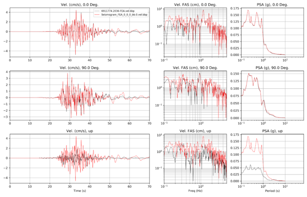
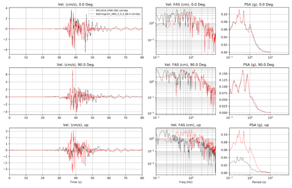
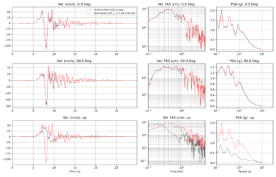
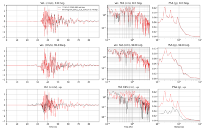
| + | Here's a comparison of a 33m run with AWP-CS, a 100m, and the BBP. | ||
| + | |||
| + | {| | ||
| + | | [[File:SCE_1D_awpcs33m_awpcs100m_bbp_lf.png|thumb|600px]] | ||
| + | |} | ||
| + | |||
| + | === Other sites, low-frequency === | ||
| + | |||
| + | {| | ||
| + | ! RO3 (LF only) | ||
| + | | [[File:RO3_1D_awp-cs_awp-oor_bbp_lf.png|thumb|600px]] | ||
| + | |- | ||
| + | ! PEL (LF only) | ||
| + | | [[File:PEL_1D_awp-cs_awp-oor_bbp_lf.png|thumb|600px]] | ||
| + | |} | ||
| + | |||
| + | |||
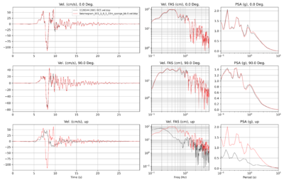
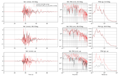
| + | === Broadband comparisons === | ||
| + | {| | ||
| + | ! Site | ||
| + | ! Broadband seismogram comparisons | ||
| + | |- | ||
| + | ! SCE | ||
| + | | [[File:SCE_1D_awpcs_bbp_bb.png|thumb|600px]] | ||
| + | |- | ||
| + | ! JGB | ||
| + | | [[File:JGB_1D_awpcs_bbp_bb.png|thumb|600px]] | ||
| + | |- | ||
| + | ! LDM | ||
| + | | [[File:LDM_1D_awpcs_bbp_bb.png|thumb|600px]] | ||
| + | |- | ||
| + | ! SPV | ||
| + | | [[File:SPV_1D_awpcs_bbp_bb.png|thumb|600px]] | ||
| + | |- | ||
| + | ! NYA | ||
| + | | [[File:NYA_1D_awpcs_bbp_bb.png|thumb|600px]] | ||
| + | |- | ||
| + | ! LBR (~45 km) | ||
| + | | [[File:LBR_1D_awpcs_bbp_bb.png|thumb|600px]] | ||
| + | |- | ||
| + | ! FEA (~80 km) | ||
| + | | [[File:FEA_1D_awpcs_bbp_bb.png|thumb|600px]] | ||
| + | |- | ||
| + | ! SBG (~105 km) | ||
| + | | [[File:SBG_1D_awpcs_bbp_bb.png|thumb|600px]] | ||
| + | |} | ||
| + | |||
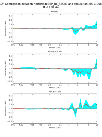
| + | === Goodness of fit plots === | ||
| + | |||
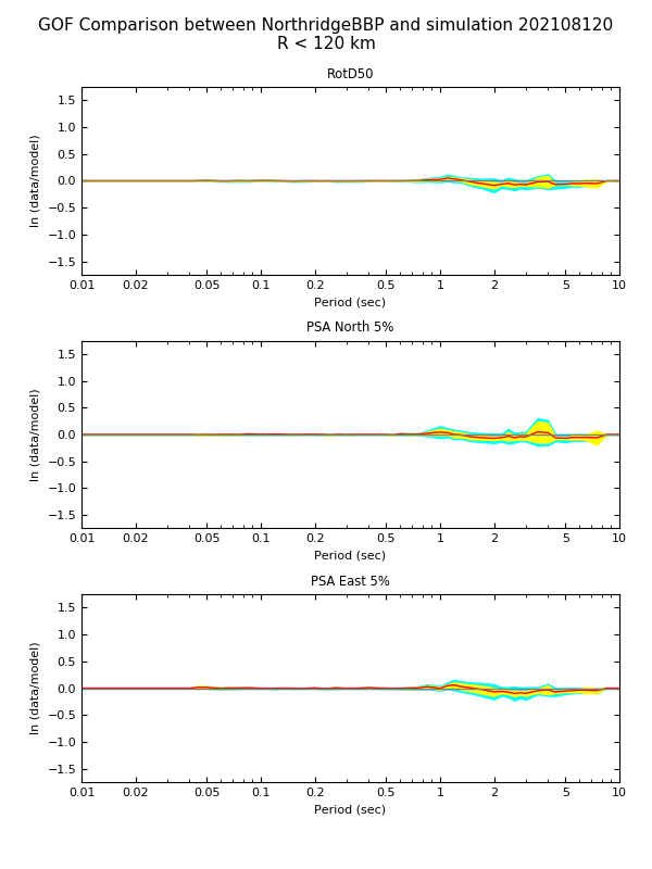
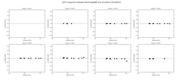
| + | Results for 10 stations, 1 realization | ||
| + | |||
| + | {| | ||
| + | | [[File:gof_Northridge_1real_10stat_rotd50.png|thumb|600px]] | ||
| + | |- | ||
| + | | [[File:gof_dist-log_Northridge_1real_10stat_rotd50.png|thumb|600px]] | ||
| + | |- | ||
| + | | [[File:gof_map_Northridge_1real_10stat_rotd50.png|thumb|600px]] | ||
| + | |} | ||
| + | |||
| + | Results for modified interpolation in jbsim3d | ||
| + | |||
| + | {| | ||
| + | | [[File:gof_modified_jbsim3d_Northridge_1real_10stat_rotd50.png|thumb|600px]] | ||
| + | |- | ||
| + | | [[File:gof_modified_jbsim3d_dist-log_Northridge_1real_10stat_rotd50.png|thumb|600px]] | ||
| + | |- | ||
| + | | [[File:gof_modified_jbsim3d_map_Northridge_1real_10stat_rotd50.png|thumb|600px]] | ||
| + | |} | ||
| + | |||
| + | === GoF for multiple realizations === | ||
| + | |||
| + | For clarity, here are the steps involved in producing the below plots. | ||
| + | |||
| + | <ol> | ||
| + | <li>Generate the 10 realizations by using a random number generator to generate 9 numbers, and create copies of the src file which is used in the BBP validation event, changing only the seed.</li> | ||
| + | <li>Produce BBP results for each of the 10 sites x 10 realizations. Note that all must be run individually so reproducibility with the random seed isn't an issue. | ||
| + | <ol style="list-style-type:lower-alpha"> | ||
| + | <li>Run the BBP workflow generator for 1 site and 1 realization to generate an XML file. This workflow includes SRF generation and site response.</li> | ||
| + | <li>Using the XML file, replace the path to the station name and the path to the src file.</li> | ||
| + | <li>Create batch submission scripts which call all 100 BBP workflows.</li> | ||
| + | </ol> | ||
| + | </li> | ||
| + | <li>Create validation events for each realization. | ||
| + | <ol style="list-style-type:lower-alpha"> | ||
| + | <li>Copy over the Northridge validation event data that ships with the BBP.</li> | ||
| + | <li>Update the data. This includes changing the event name, updating the src file, updating the stl file to filter at the correct frequencies, and stage in the output acceleration data from the BBP runs for the validation event to use as an 'observation'.</li> | ||
| + | </ol> | ||
| + | </li> | ||
| + | <li>Produce CyberShake results for each of the 10 sites. | ||
| + | <ol style="list-style-type:lower-alpha"> | ||
| + | <li>Create a new source in the ERF, in which each realization is a separate rupture of that source.</li> | ||
| + | <li>Extract the rupture geometry from one of the realizations, to obtain the list of points the SGTs should be saved for.</li> | ||
| + | <li>Generate a CyberShake volume oriented N/S/E/W which contains the Northridge rupture surface, the site of interest, is 64 km deep, and uses 30 km of padding.</li> | ||
| + | <li>Generate a velocity mesh using the 24-layer model provided by Rob, which is a post-processed version of the LA Basin 14-layer model included with the BBP.</li> | ||
| + | <li>Run the original version of the AWP code ('AWP-CS'), using velocity insertion of a source low-pass filtered at 2 Hz, for 30 seconds (unless it's a distance site, in which case we run longer)</li> | ||
| + | <li>Run the post-processing code for the 10 realizations.</li> | ||
| + | <li>Run the broadband steps (high-frequency synthesis, low-frequency site response, and merge) for each of the 10 realizations.</li> | ||
| + | </ol> | ||
| + | </li> | ||
| + | <li>Perform goodness-of-fit, using CyberShake as the simulation and BBP as the reference. | ||
| + | <ol style="list-style-type:lower-alpha"> | ||
| + | <li>For each realization: | ||
| + | <ol> | ||
| + | <li>Create a temporary directory for the CyberShake results.</li> | ||
| + | <li>Stage in the CyberShake results for all 10 sites</li> | ||
| + | <li>Use BBP helper scripts to create a simulation ID and stage the CyberShake results to that directory.</li> | ||
| + | <li>Run the BBP to generate an XML file which will perform GoF (details at [[New_BBP_Validation_Package]])</li> | ||
| + | <li>Run using the XML file to generate the GoF comparisons and plots.</li> | ||
| + | </ol> | ||
| + | </li> | ||
| + | </ol> | ||
| + | </li> | ||
| + | </ol> | ||
| + | |||
| + | {| border="1" | ||
| + | ! Realization !! GoF plot !! Ratio by distance | ||
| + | |- | ||
| + | | 1 || [[File:gof_modified_jbsim3d_Northridge_1real_10stat_rotd50.png|thumb|600px]] || [[File:gof_modified_jbsim3d_dist-log_Northridge_1real_10stat_rotd50.png|thumb|600px]] | ||
| + | |- | ||
| + | | 2 || [[File:gof_Northridge_2real_10stat_rotd50.png|thumb|600px]] || [[File:gof_dist-log_Northridge_2real_10stat_rotd50.png|thumb|600px]] | ||
| + | |- | ||
| + | | 3 || [[File:gof_Northridge_3real_10stat_rotd50.png|thumb|600px]] || [[File:gof_dist-log_Northridge_3real_10stat_rotd50.png|thumb|600px]] | ||
| + | |- | ||
| + | | 4 || [[File:gof_Northridge_4real_10stat_rotd50.png|thumb|600px]] || [[File:gof_dist-log_Northridge_4real_10stat_rotd50.png|thumb|600px]] | ||
| + | |- | ||
| + | | 5 || [[File:gof_Northridge_5real_10stat_rotd50.png|thumb|600px]] || [[File:gof_dist-log_Northridge_5real_10stat_rotd50.png|thumb|600px]] | ||
| + | |- | ||
| + | | 6 || [[File:gof_Northridge_6real_10stat_rotd50.png|thumb|600px]] || [[File:gof_dist-log_Northridge_6real_10stat_rotd50.png|thumb|600px]] | ||
| + | |- | ||
| + | | 7 || [[File:gof_Northridge_7real_10stat_rotd50.png|thumb|600px]] || [[File:gof_dist-log_Northridge_7real_10stat_rotd50.png|thumb|600px]] | ||
| + | |- | ||
| + | | 8 || [[File:gof_Northridge_8real_10stat_rotd50.png|thumb|600px]] || [[File:gof_dist-log_Northridge_8real_10stat_rotd50.png|thumb|600px]] | ||
| + | |- | ||
| + | | 9 || [[File:gof_Northridge_9real_10stat_rotd50.png|thumb|600px]] || [[File:gof_dist-log_Northridge_9real_10stat_rotd50.png|thumb|600px]] | ||
| + | |- | ||
| + | | 10 || [[File:gof_Northridge_10real_10stat_rotd50.png|thumb|600px]] || [[File:gof_dist-log_Northridge_10real_10stat_rotd50.png|thumb|600px]] | ||
| + | |} | ||
| + | |||
| + | Combined goodness-of-fit | ||
| + | |||
| + | {| | ||
| + | | [[File:gof_Northridge_aggregate_10real_10stat_rotd50.png|thumb|600px]] | ||
| + | |} | ||
| + | |||
| + | === 33m tests === | ||
| + | |||
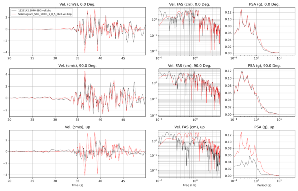
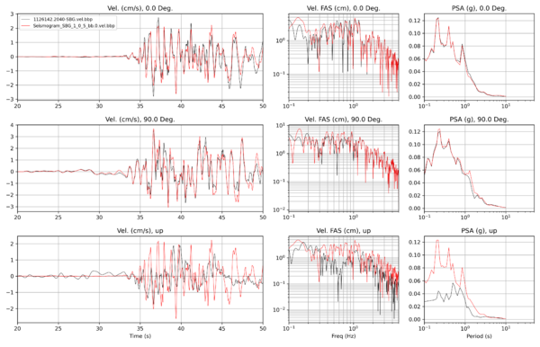
| + | We modified the grid spacing from 100m to 33.333m to see what impact it has on the BBP/CS comparisons. To simplify the comparisons, results here are for 1 Northridge realization, realization 6. | ||
| + | |||
| + | {| | ||
| + | ! Site !! 100m !! 33m | ||
| + | |- | ||
| + | | SCE || [[File:SCE_1D_nrR6_100m_bbp_v_cs.png|thumb|600px]] || [[File:SCE_1D_nrR6_33m_bbp_v_cs.png|thumb|600px]] | ||
| + | |- | ||
| + | | SBG || [[File:SBG_1D_nrR6_100m_bbp_v_cs.png|thumb|600px]] || [[File:SBG_1D_nrR6_33m_bbp_v_cs.png|thumb|600px]] | ||
| + | |} | ||
| + | |||
| + | === Expanded buffer layer tests === | ||
| + | |||
| + | When calculating the size of the CyberShake volume, we construct a volume large enough to contain the site and all the fault surfaces, then pad it on all sides by 30 km. We modified the buffer zone to be larger, 50 km. | ||
| + | |||
| + | {| | ||
| + | ! Site !! 30 km buffer zone !! 50 km buffer zone | ||
| + | |- | ||
| + | | SCE || [[File:SCE_1D_nrR6_30km_bbp_v_cs.png|thumb|600px]] || [[File:SCE_1D_nrR6_50km_bbp_v_cs.png|thumb|600px]] | ||
| + | |- | ||
| + | | SBG || [[File:SBG_1D_nrR6_30km_bbp_v_cs.png|thumb|600px]] || [[File:SBG_1D_nrR6_50km_bbp_v_cs.png|thumb|600px]] | ||
| + | |} | ||
| + | |||
| + | We then performed additional tests, deepening the volume to 80 km, increasing the padding to 60 km, and also increasing the number of grid points in the boundary condition sponge zone from 50 to 80. Below are comparisons with the original results, including GoF for site SBG. | ||
| + | |||
| + | All plots are for Northridge realization 6. | ||
| + | |||
| + | {| | ||
| + | ! Site (spacing) !! 64 km deep, 30 km padding, 50 point sponge zone !! GoF for original configuration !! 80 km deep, 60 km padding, 80 point sponge zone !! GoF for modified configuration !! 80 km deep, 60 km padding, 240 point sponge zone | ||
| + | |- | ||
| + | ! SCE (100m) | ||
| + | | [[File:SCE_1D_nrR6_bbp_v_100m_cs.png|thumb|400px]] || || [[File:SCE_1D_nrR6_bbp_v_100m_sponge_cs.png|thumb|400px]] || || [[File:SCE_1D_nrR6_bbp_v_33m_cs_240sponge.png|thumb|400px]] | ||
| + | |- | ||
| + | ! SCE (33m) | ||
| + | | [[File:SCE_1D_nrR6_bbp_v_33m_cs.png|thumb|400px]] || || [[File:SCE_1D_nrR6_bbp_v_33m_sponge_cs.png|thumb|400px]] || | ||
| + | |- | ||
| + | ! SBG (100m) | ||
| + | | [[File:SBG_1D_nrR6_bbp_v_100m_cs.png|thumb|400px]] || [[File:gof_SBG_1D_nrR6_100m_cs.png|thumb|400px]] || [[File:SBG_1D_nrR6_bbp_v_100m_cs_sponge.png|thumb|400px]] || [[File:gof_SBG_1D_nrR6_100m_cs_sponge.png|thumb|400px]] | ||
| + | |- | ||
| + | ! SBG (33m) | ||
| + | | [[File:SBG_1D_nrR6_bbp_v_33m_cs.png|thumb|400px]] || [[File:gof_SBG_1D_nrR6_33m_cs.png|thumb|400px]] || [[File:SBG_1D_nrR6_bbp_v_33m_cs_sponge.png|thumb|400px]] || [[File:gof_SBG_1D_nrR6_33m_cs_sponge.png|thumb|400px]] | ||
| + | |} | ||
| + | |||
| + | We tried SBG for both 100m and 33m, saving the SGTs at the same dt as the BBP (0.1s). | ||
| + | |||
| + | {| | ||
| + | | SBG (100m), sim dt=0.005, SGT dt=0.1 | ||
| + | | [[File:SBG_1D_nrR6_bbp_v_33m_dt0.1.png|thumb|400px]] | ||
| + | |- | ||
| + | | SBG (33m), sim dt=0.001, SGT dt=0.1 | ||
| + | | [[File:SBG_1D_nrR6_bbp_v_100m_dt0.1.png|thumb|400px]] | ||
| + | |} | ||
| + | |||
| + | === Northridge, 38 stations === | ||
| + | |||
| + | We ran CyberShake and the BBP for 10 realizations for the 38 distinct stations listed [[Media:northridge_stations.kml|here]]. Note that 2006-PAC and 2007-PUL are colocated, so we only ran one. Below are goodness-of-fit and scatterplot GOF results. | ||
| + | |||
| + | {| | ||
| + | ! Realization !! GoF plot !! GoF scatterplot | ||
| + | |- | ||
| + | ! 2 | ||
| + | | [[File:gof_Northridge_2real_38stat_rotd50.png|thumb|600px]] | ||
| + | | [[File:gof_Northridge_2real_38stat_scatter.png|thumb|600px]] | ||
| + | |- | ||
| + | ! 3 | ||
| + | | [[File:gof_Northridge_3real_38stat_rotd50.png|thumb|600px]] | ||
| + | | [[File:gof_Northridge_3real_38stat_scatter.png|thumb|600px]] | ||
| + | |- | ||
| + | ! 4 | ||
| + | | [[File:gof_Northridge_4real_38stat_rotd50.png|thumb|600px]] | ||
| + | | [[File:gof_Northridge_4real_38stat_scatter.png|thumb|600px]] | ||
| + | |- | ||
| + | ! 5 | ||
| + | | [[File:gof_Northridge_5real_38stat_rotd50.png|thumb|600px]] | ||
| + | | [[File:gof_Northridge_5real_38stat_scatter.png|thumb|600px]] | ||
| + | |- | ||
| + | ! 6 | ||
| + | | [[File:gof_Northridge_6real_38stat_rotd50.png|thumb|600px]] | ||
| + | | [[File:gof_Northridge_6real_38stat_scatter.png|thumb|600px]] | ||
| + | |- | ||
| + | ! 7 | ||
| + | | [[File:gof_Northridge_7real_38stat_rotd50.png|thumb|600px]] | ||
| + | | [[File:gof_Northridge_7real_38stat_scatter.png|thumb|600px]] | ||
| + | |- | ||
| + | ! 8 | ||
| + | | [[File:gof_Northridge_8real_38stat_rotd50.png|thumb|600px]] | ||
| + | | [[File:gof_Northridge_8real_38stat_scatter.png|thumb|600px]] | ||
| + | |- | ||
| + | ! 9 | ||
| + | | [[File:gof_Northridge_9real_38stat_rotd50.png|thumb|600px]] | ||
| + | | [[File:gof_Northridge_9real_38stat_scatter.png|thumb|600px]] | ||
| + | |- | ||
| + | ! 10 | ||
| + | | [[File:gof_Northridge_10real_38stat_rotd50.png|thumb|600px]] | ||
| + | | [[File:gof_Northridge_10real_38stat_scatter.png|thumb|600px]] | ||
|} | |} | ||
| Line 491: | Line 761: | ||
*[[CyberShake]] | *[[CyberShake]] | ||
*[[Broadband Platform]] | *[[Broadband Platform]] | ||
| + | *[[New BBP Validation Package]] | ||
Latest revision as of 21:56, 25 August 2023
This page documents our initial CyberShake Broadband Platform verification work, running the BBP validation events through CyberShake.
Contents
Events
The BBP has support for the following events. We plan to run the ones in bold:
- Alum Rock Mw 5.45
- Chino Hills Mw 5.39
- Hector Mine Mw 7.13
- Landers Mw Mw 7.22*
- Loma Prieta Mw 6.94
- North Palm Springs Mw 6.12
- Northridge Mw 6.73
- Parkfield Mw 6.0
- Ridgecrest A Mw 6.47
- Ridgecrest B Mw 5.4
- Ridgecrest C Mw 7.08*
- San Simeon Mw 6.6*
- Whittier Narrows Mw 5.89
Verification and Validation
Planned process will involve verification and validation stages.
- Verification: Compare CyberShake broadband seismograms to Broadband Platform seismograms
- Validation: Compare CyberShake broadband seismograms to observed seismograms
Verification Process
Validation Process
For each of the 5 BBP validation events listed above, go through the following process:
- Run the BBP validation event with the Graves & Pitarka modules to produce BBP results for comparison.
- Review the BBP validation data for the event, including station list and seismogram files and validation results from GP method for this event.
- Identify about 10 stations from the BBP station list that have observed seismograms to run in CyberShake.
- Modify station list low-pass filter to 50 Hz.
- Use the Vs30 values from the BBP station list for both the low-frequency and high-frequency site response in CyberShake, for consistency.
- We will use CVM-S4.26.M01 as the velocity model for CyberShake.
- Run one realization using the SRF file which is generated by the BBP when run with one realization.
- Create an ERF in the CyberShake database containing all the validation events, with a unique source and rupture ID for each one.
- Save the SGTs in case we want to run additional realizations later.
- To interface with the BBP tools for generating data products, convert the CyberShake seismograms into BBP format seismograms
Data Products
The CyberShake method calculates two component seismograms. Broadband platform supports three component seismograms. We will convert CyberShake 2 components to 3 components by duplicating the N/S component in the vertical component data.
We will produce the following data products to compare CyberShake results with BBP results:
- ts_process plot, comparing traces and response spectra.
- RotD50 comparison plots
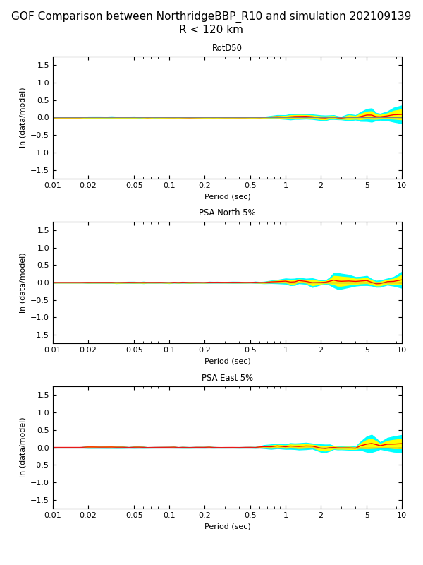
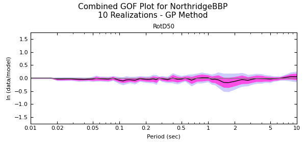
- Goodness-of-fit bias plots
- Map of GoF, by station
Northridge
A KML of the Northridge stations is available here. Selected stations are in orange. The BBP station list file for these stations is available here.
We made the following modifications to the default BBP platform to support better comparison to the BB CS results:
- Changed the BBP LF and HF seismogram length to 500 sec / 50,000 timesteps
- Modified the filtering so the merge frequency is 1.0 Hz and phase=0
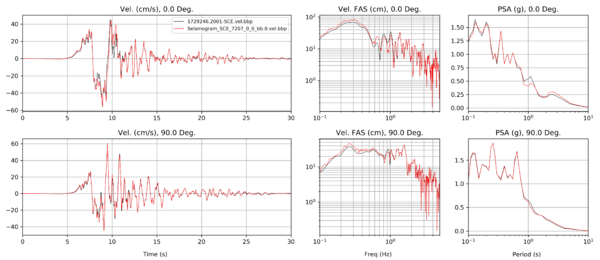
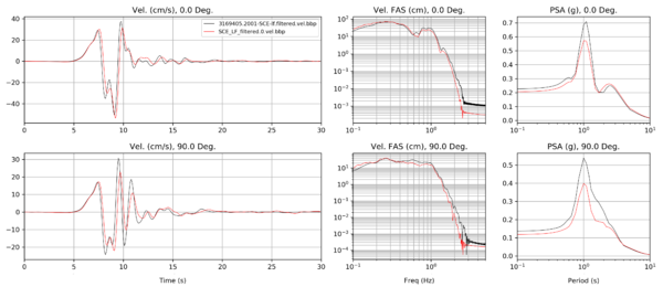
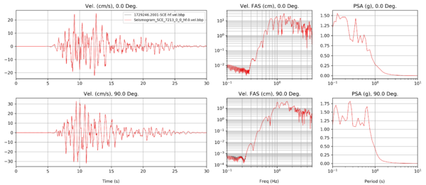
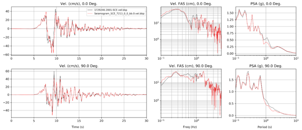
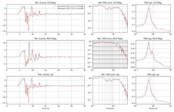
3D comparisons
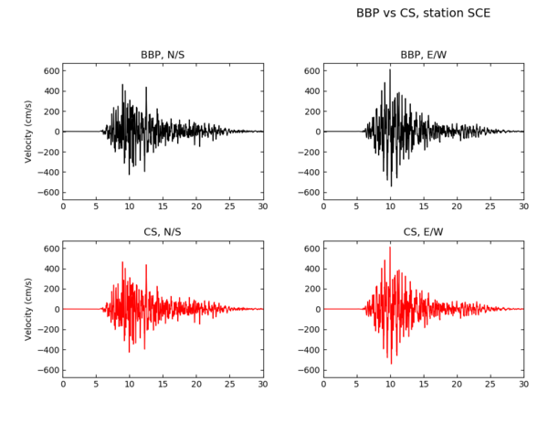
Below are comparisons using the CVM-S4.26.M01 model in CyberShake.
| Stage | Seismogram comparison |
|---|---|
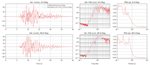
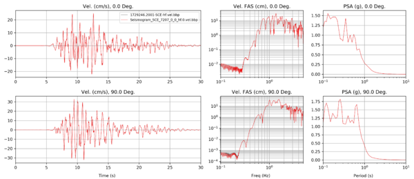
| Filtered high-frequency acceleration with site response |
|
| Low-frequency velocity | |
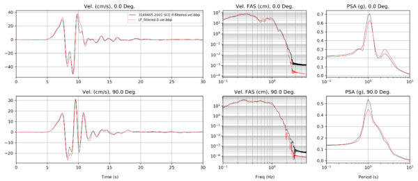
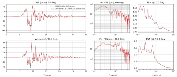
| Broadband velocity |
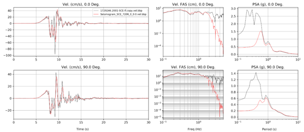
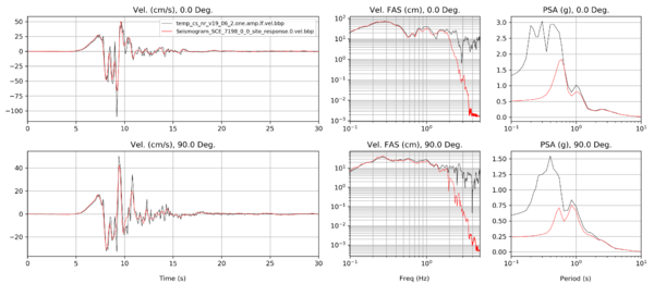
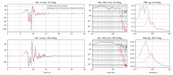
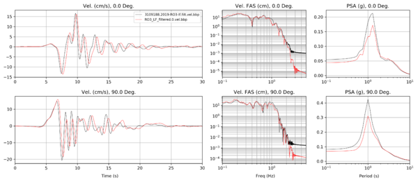
BBP LA Basin 1D comparisons
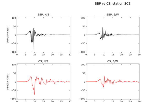
Below are comparisons using the BBP 1D LA Basin model in CyberShake with no interpolation. We also:
- Modified the CyberShake filtering scheme to match the BBP filtering scheme, which uses a high-pass filter for the HF at around 0.89 Hz and a low-pass filter for the LF at about 1.11 Hz.
- Modified the CyberShake low-frequency site response to use the high-frequency PGA values, consistent with the BBP approach.
We ran SCE with both the original 1D model, and a modified version (File:Modified nr02-vs500.txt)
| Stage | BBP vs CS, original 1D | BBP vs CS, modified 1D |
|---|---|---|
| Low-frequency (velocity) | ||
| Low-frequency with site response (velocity) |
||
| Low-frequency with site response and filtering (velocity) |
||
| High-frequency with site response and filtering (velocity) |
||
| Broadband results (velocity) |
Comparable dt
We reran our comparisons with the same dt (0.1) for SCE in CyberShake and the BBP:
| Stage | BBP vs CS, original 1D | |
|---|---|---|
| Low-frequency with site response and filtering (velocity) |
||
| High-frequency with site response and filtering (velocity) |
||
| Broadband results (velocity) |
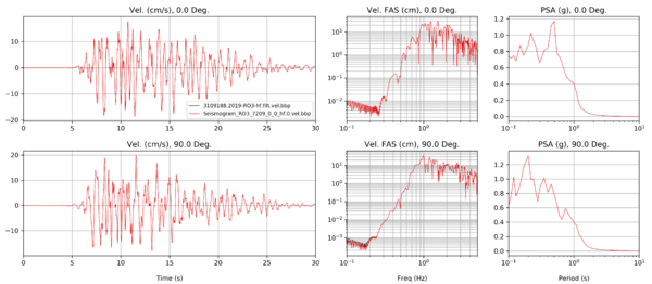
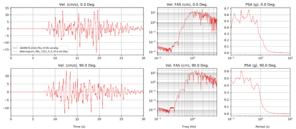
Other sites
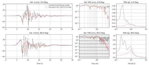
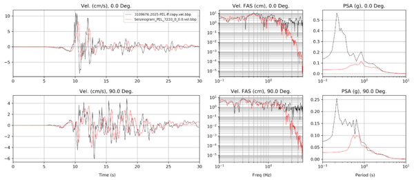
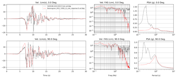
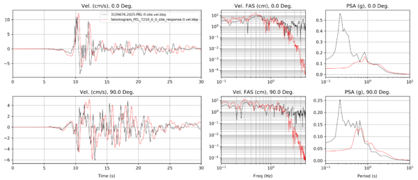
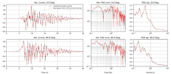
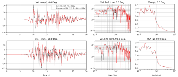
| RO3 (5/170 interchange) | PEL (Santa Monica/Highland) | |
|---|---|---|
| Low-frequency (velocity) | ||
| Low-frequency with site response (velocity) |
||
| Low-frequency with site response and filtering (velocity) |
||
| High-frequency with site response and filtering (velocity) |
||
| Broadband results (velocity) |
Halfspace comparisons
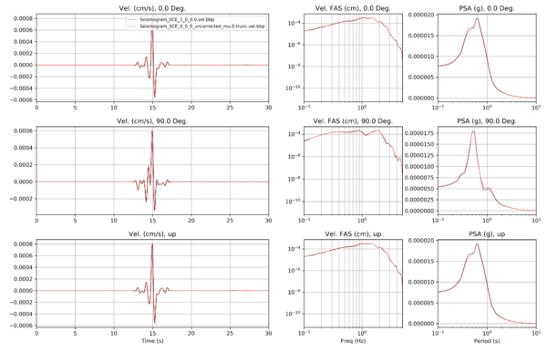
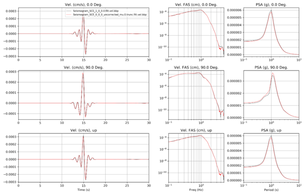
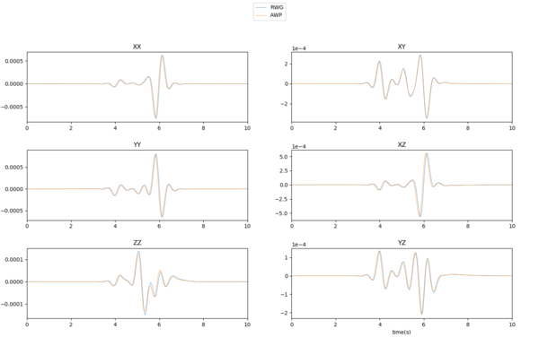
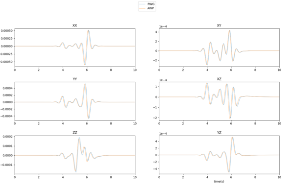
Seismograms
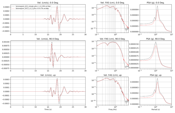
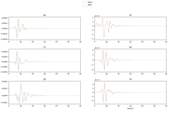
Point source. Red = AWP, Black = RWG.
| Unfiltered | |
|---|---|
| Filtered |
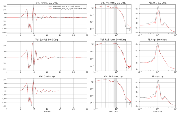
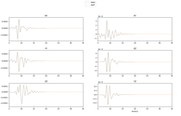
Northridge BBP validation event. Red = AWP, Black = RWG.
| Unfiltered | |
|---|---|
| Filtered |
SGTs
| X-component | Y-component | |
|---|---|---|
| Adjusted mu in AWP | ||
| Unadjusted mu in AWP |
Uncorrected mu
Modified 1D velocity model
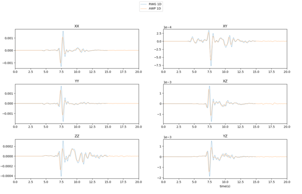
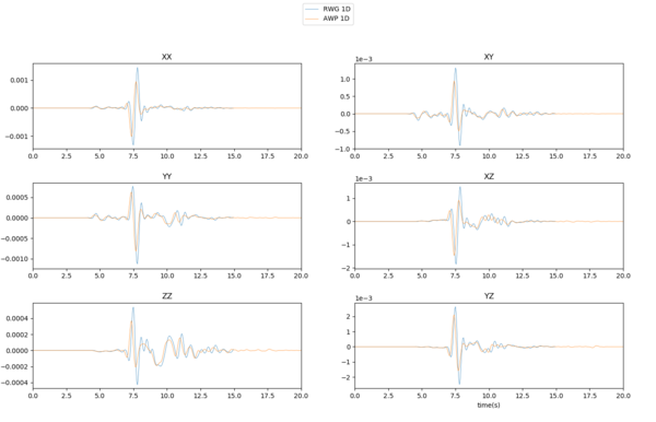
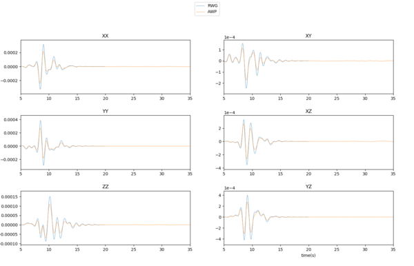
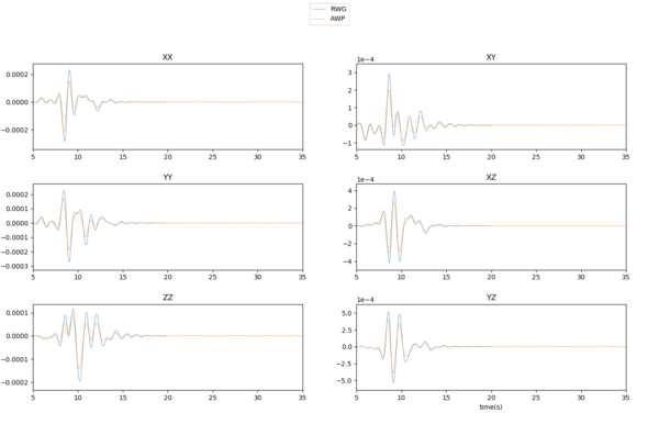
RWG and AWP SGTs, using SGT headers with uncorrected mu values
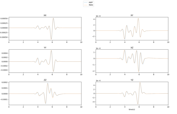
Filtered seismograms (red = AWP, black = RWG)
| Point source | |
|---|---|
| Northridge |
SGTs (red = AWP, black = RWG)
| X | Y |
|---|---|
1Hz source plots
To reduce ringing effects, we started using an impulse low-pass filtered at 1 Hz.
All the plots below are of SGTs.
Slow halfspace
The plots below were calculated using a halfspace model with Vp=1500, Vs=750, rho=2200.
Qs=37.5, Qp=75.0
| X | Y |
|---|---|
Qs=10000, Qp=20000
| X | Y |
|---|---|
4-layered model
Next we ran with a 4-layered model:
Thickness(km)   Vp      Vs      rho
0.2500          2.4000  1.0000  2.2500
0.7000          3.7000  1.8000  2.4500
1.5000          4.7500  2.4000  2.6000
2.5000          5.4000  3.0000  2.6500
999.00          6.2000  3.5000  2.7200
Qs=10000, Qp=20000
| X | Y |
|---|---|
Qs=0.05Vs, Qp=2Qs
| X | Y |
|---|---|
Qs=0.05Vs, Qp=2Qs
Unadjusted mu and lambda used for stress->strain conversion. This was accomplished by removing adjustment factors in the SGT kernel.
| Depth | X | Y |
|---|---|---|
| Shallow (5 km) | ||
| Deep (15 km) |
12-layered model
   Vp      Vs      rho         Depth to layer bottom (km)
  2.4000   1.0000   2.2500     0.250001
  3.1000   1.4000   2.3000     0.450001
  3.3495   1.5560   2.3750     0.550001
  3.7000   1.8000   2.4500     0.950001
  3.9190   1.9285   2.5125     1.050001
  4.2000   2.1000   2.5750     1.450001
  4.4483   2.2343   2.5875     1.550001
  4.7500   2.4000   2.6000     2.450001
  4.9150   2.5565   2.6100     2.550001
  5.1000   2.7500   2.6200     3.450001
  5.2426   2.8661   2.6350     3.550001
  5.4000   3.0000   2.6500     4.950001
  6.2000   3.5000   2.7200     9999.999999
Qs=0.05Vs, Qp=2Qs
Unadjusted mu and lambda used for stress->strain conversion.
| Depth | X | Y |
|---|---|---|
| Shallow (5 km) | ||
| Deep (15 km) |
14-layered model
   Vp      Vs      rho      Depth to layer bottom (km)
  1.6447   0.5378   2.0600     0.050001
  1.8893   0.7115   2.1500     0.150001
  2.3653   0.9766   2.2500     0.250001
  3.1000   1.4000   2.3000     0.450001
  3.3495   1.5560   2.3750     0.550001
  3.7000   1.8000   2.4500     0.950001
  3.9190   1.9285   2.5125     1.050001
  4.2000   2.1000   2.5750     1.450001
  4.4483   2.2343   2.5875     1.550001
  4.7500   2.4000   2.6000     2.450001
  4.9150   2.5565   2.6100     2.550001
  5.1000   2.7500   2.6200     3.450001
  5.2426   2.8661   2.6350     3.550001
  5.4000   3.0000   2.6500     4.950001
  6.2000   3.5000   2.7200  9999.999999
Qs=0.05Vs, Qp=2Qs
Unadjusted mu and lambda used for stress->strain conversion.
| Depth | X | Y |
|---|---|---|
| Shallow (5 km) | ||
| Deep (15 km) |
Forward/Reverse Tests
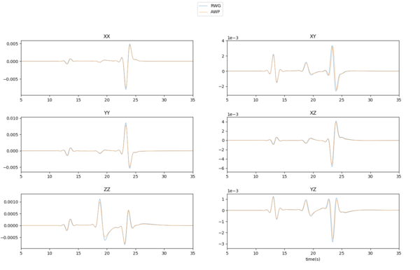
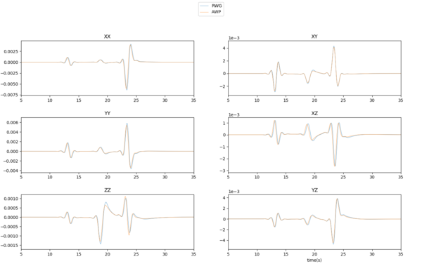
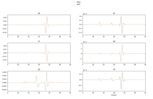
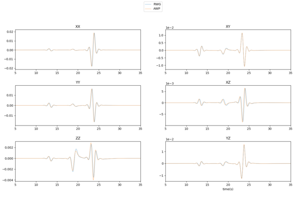
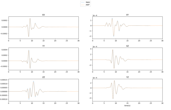
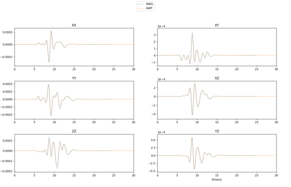
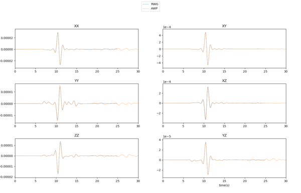
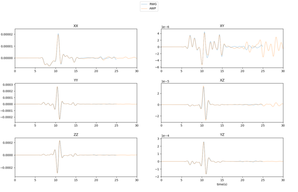
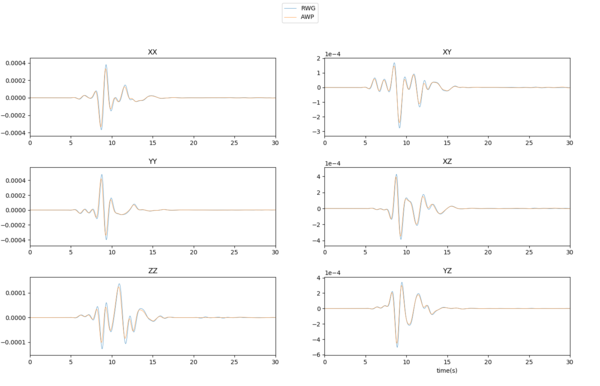
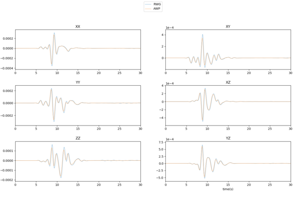
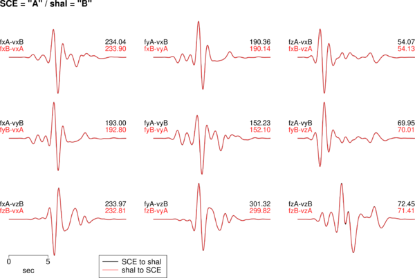
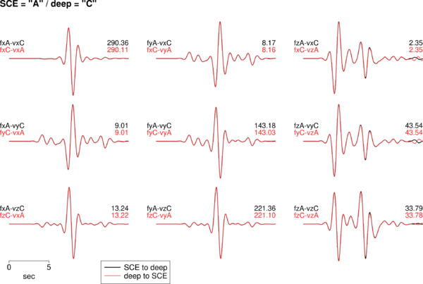
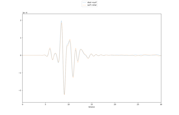
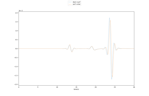
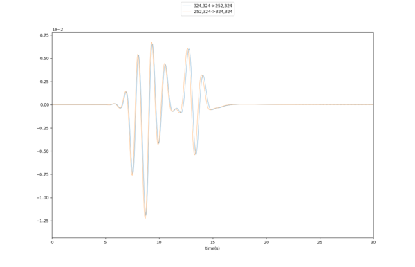
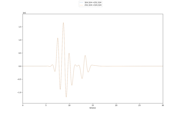
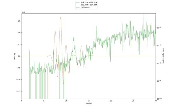
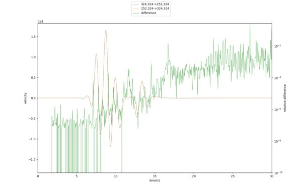
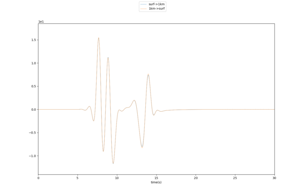
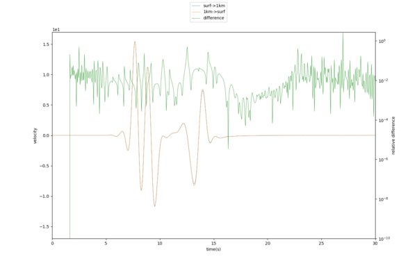
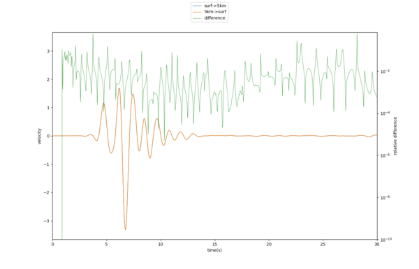
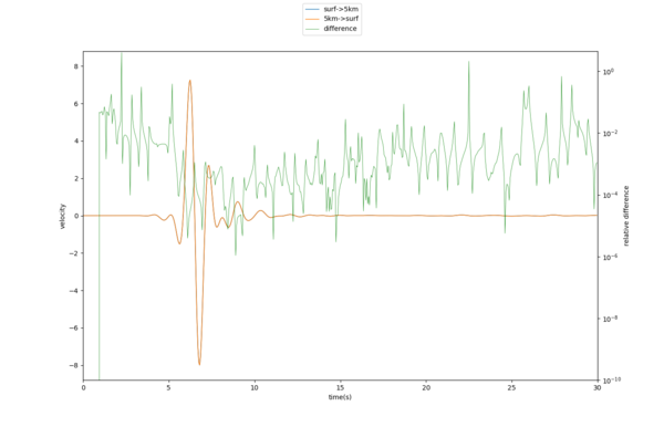
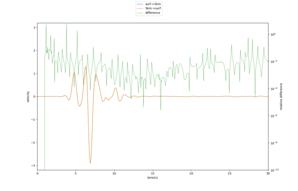
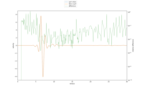
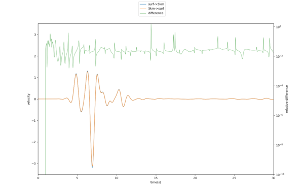
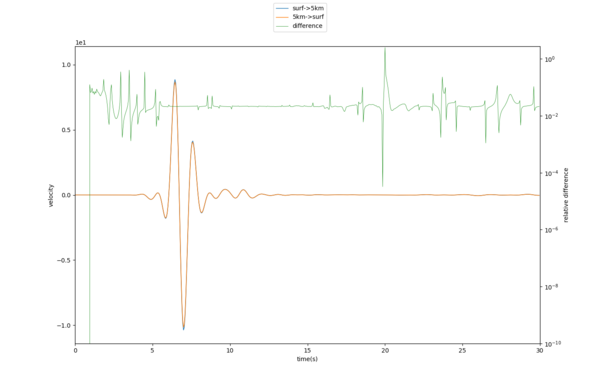
To narrow down potential issues further, we performed a series of forward/reverse tests. In these, we place a force at one location and observe the velocities at another, then place a force at the 2nd location and observe the velocities at the first. As long as the correct components are being compared, the resulting seismograms should be very similar.
Results from Rob's 4th-order code (14-layer model), using the points at 5 km and the surface, and 15 km depth and the surface.
| Depth | Results |
|---|---|
| 5 km | |
| 15 km |
Rob repeated the experiment with 2nd-order operators and got agreement to floating-point error.
Using the AWP-CS code, we got the following results. We averaged the Z=1 and Z=2 layers to correctly get the free surface velocities. For some reason, one of the seismograms needs to be inverted in order to match correctly.
| Model | Results for 5 km/source pair |
|---|---|
| 14 layer | |
| 12 layer | | |
| 4 layer | |
| halfspace |
Velocity source insertion
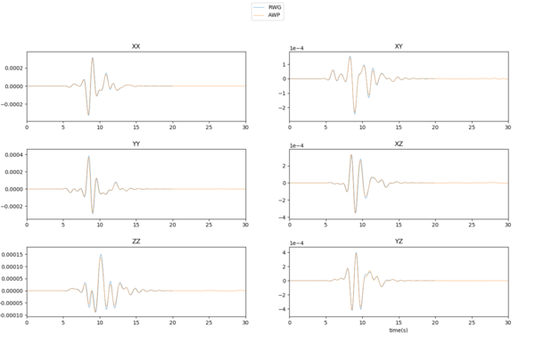
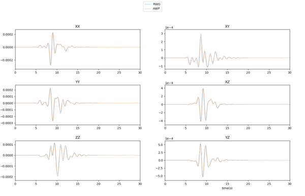
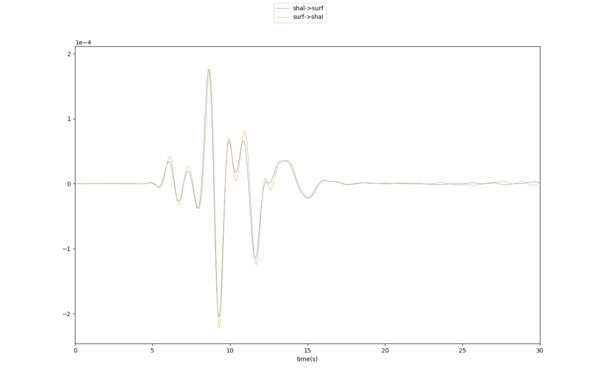
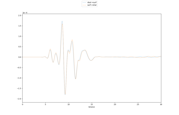
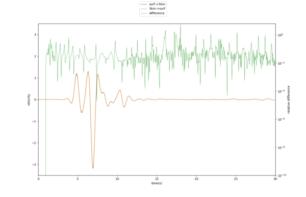
We determined that the offset is due to the way the AWP staggered grid is set up. The normal stresses are in the center of the grid cell, but the X velocity is in the center of the side, in the +x direction. So inserting a source at location A and recording velocities at location B is actually recording velocities at B+.5, and doing the reverse tests means velocities are measured at A+.5. So in the first test, the distance traveled is (B+.5)-A = (B-A)+.5, and in the second it's B-(A+.5) = (B-A)-.5, a difference of 1 grid point. If the force is inserted by modifying velocities,
To illustrate this, the plots below show the same test with a stress insertion and a velocity insertion. Both points have the same Y and Z indices (depth=1km), only the X is varied.
| Stress insertion | |
|---|---|
| Velocity insertion |
Here's a plot of the relative differences:
We also tried increasing Q to 1e10:
Since the above results looked good, we tried moving one of the points to the surface:
The differences in the late arrivals are ~3%.
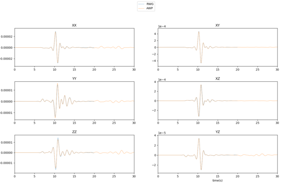
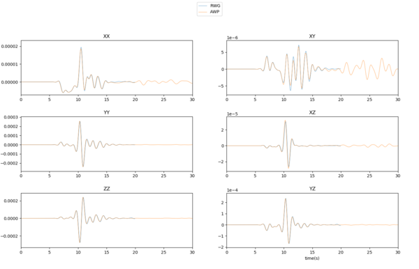
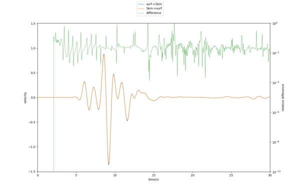
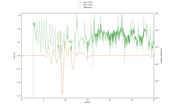
We repeated these velocity insertion tests for the 4, 12, and 14-layer models, with one point at the surface and one point at depth.
| Model | X results | Y results |
|---|---|---|
| 4-layer | ||
| 12-layer | ||
| 14-layer |
I ran a model at 33m resolution. Here are the difference plots, and comparison to the 100m model, for a halfspace.
Kim made some updates to the symmetries in the kernel. I reran the 14-layer tests with the new kernel.
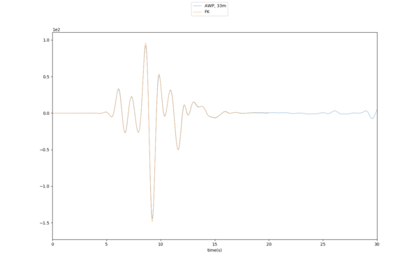
We recomputed results using 100m and 33m spacing, and compared them to the FK results for the 14-layer model. We chose the AWP points (432, 365, 1) and (317, 453, 52) in the 100m run and (1294, 1093, 1) and (948, 1362, 154) in the 33m run.
| 100m self-reciprocity, X component | |
|---|---|
| 33m self-reciprocity, X component | |
| 100m vs 33m | |
| 33m vs FK |
SGT Tests
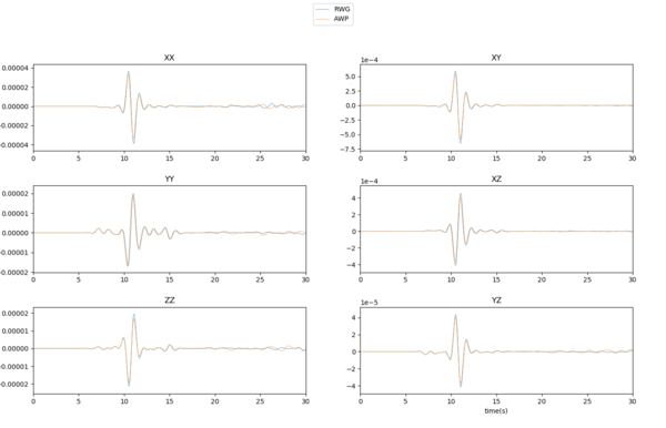
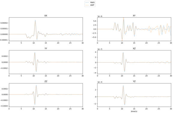
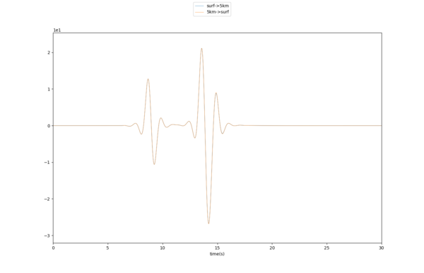
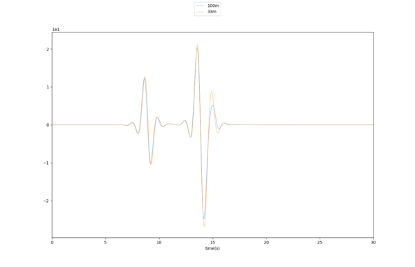
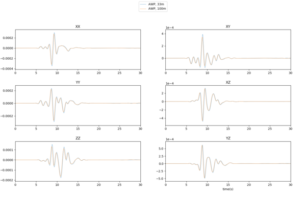
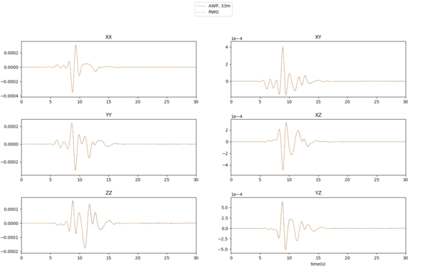
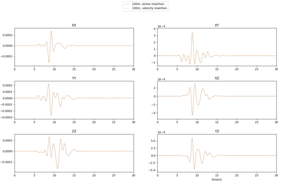
Using the 14-layer model, we ran tests to generate SGTs at 100m and 33.333m grid spacing, using both velocity and stress insertion
| AWP 100m vs RWG 100m, X component | |
|---|---|
| AWP 33m vs AWP 100m, X component | |
| AWP 33m vs RWG 100m, X component | |
| AWP 100m velocity insertion vs AWP 100m stress insertion, X component |
BBP Comparisons
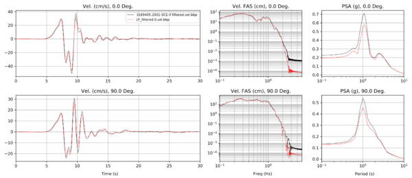
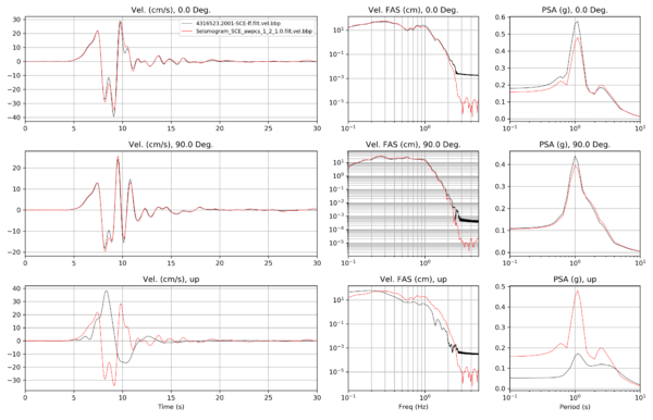
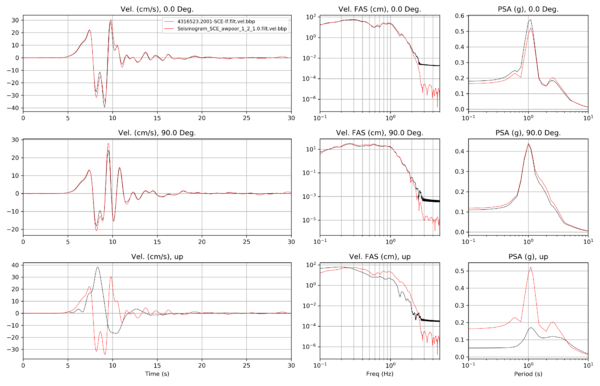
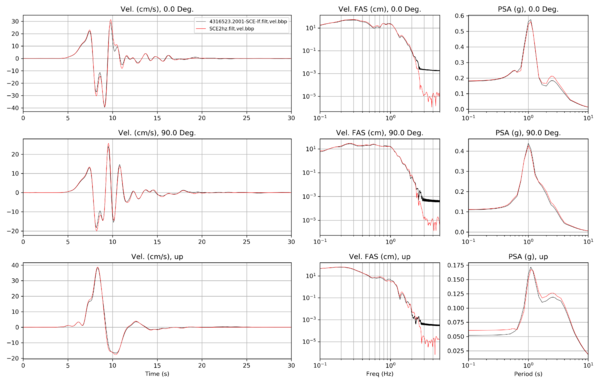
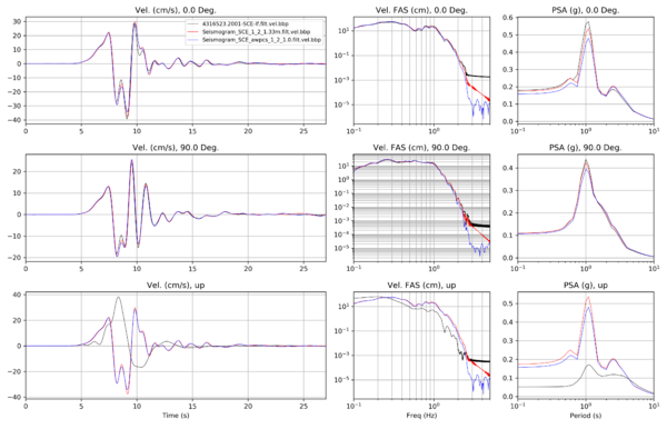
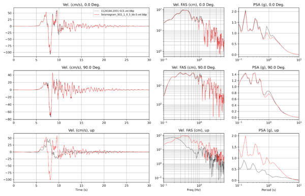
For these comparisons, we used the 14-layer model in the BBP, and a 24-layer pre-processed version of this model better for finite difference codes.
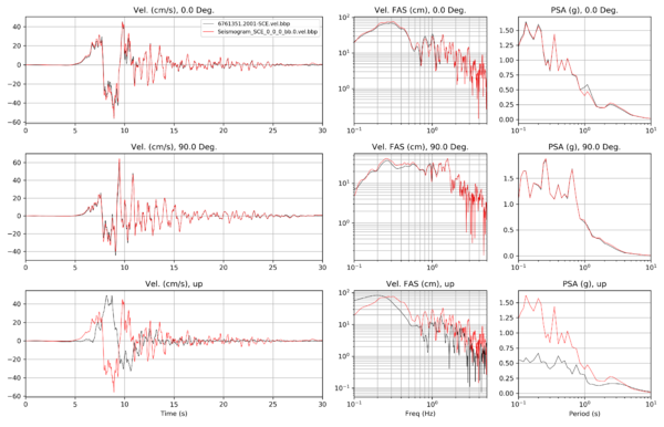
Site SCE
| BBP vs AWP-CS | |
|---|---|
| BBP vs AWP-OOR (modified source insertion) | |
| BBP vs RWG reciprocity |
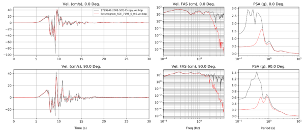
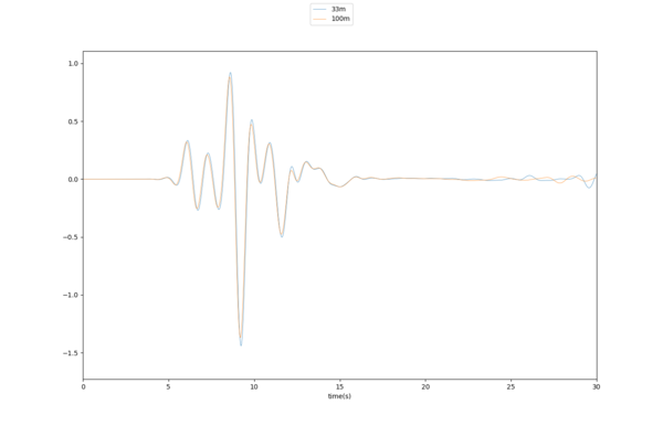
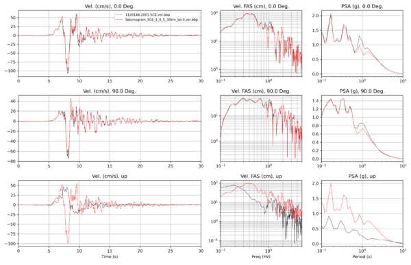
Here's a comparison of a 33m run with AWP-CS, a 100m, and the BBP.
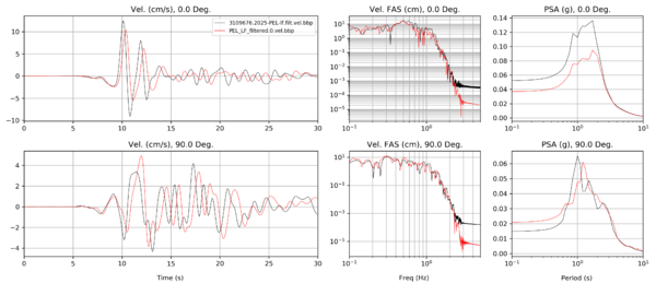
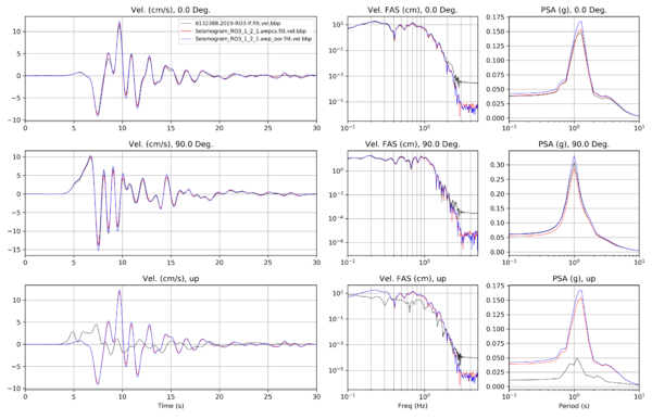
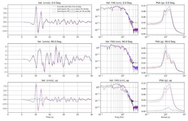
Other sites, low-frequency
| RO3 (LF only) | |
|---|---|
| PEL (LF only) |
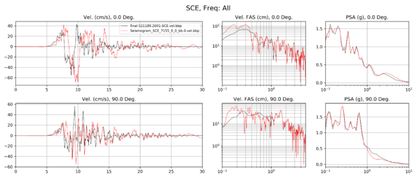
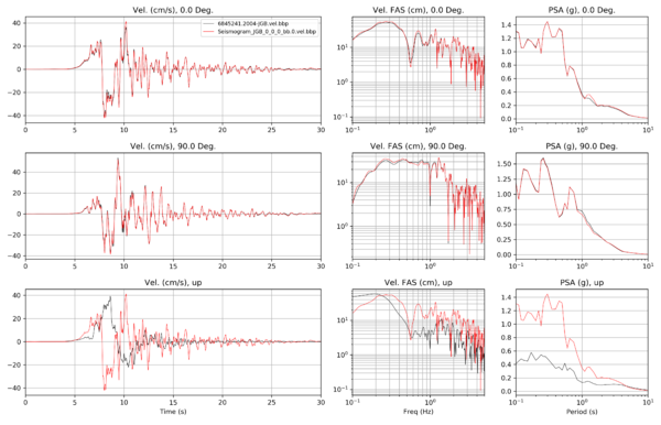
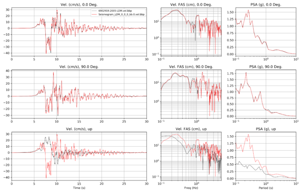
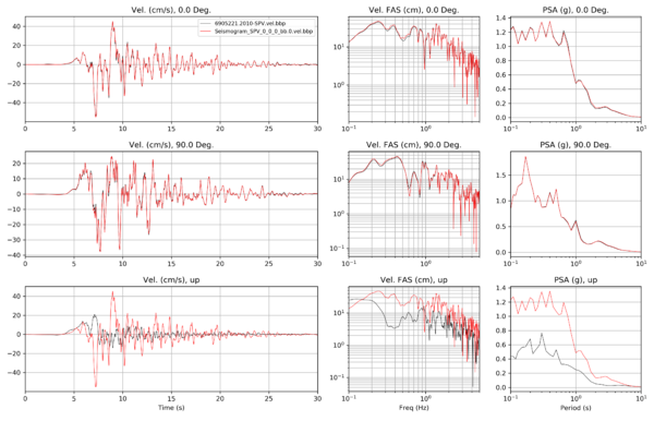
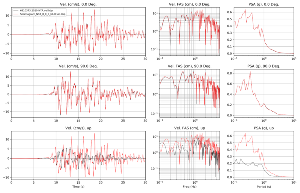
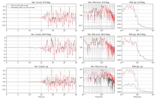
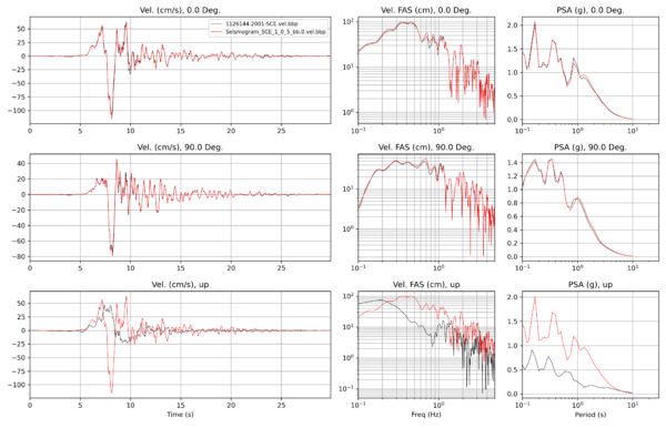
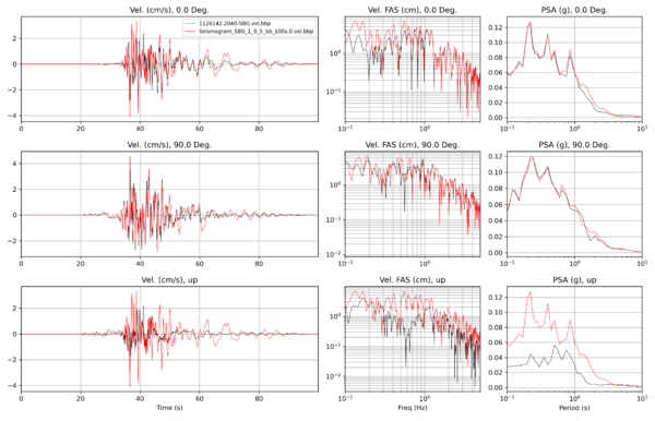
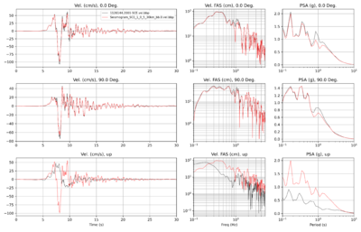
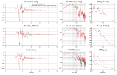
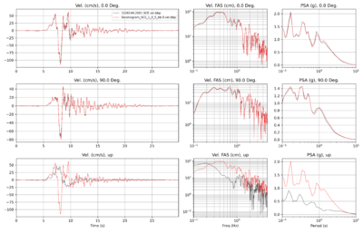
Broadband comparisons
| Site | Broadband seismogram comparisons |
|---|---|
| SCE | |
| JGB | |
| LDM | |
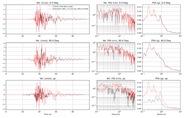
| SPV | |
| NYA | |
| LBR (~45 km) | |
| FEA (~80 km) | |
| SBG (~105 km) |
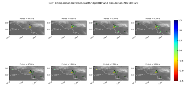
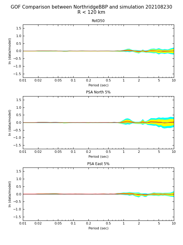
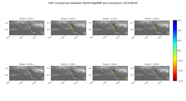
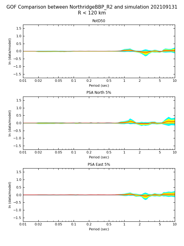
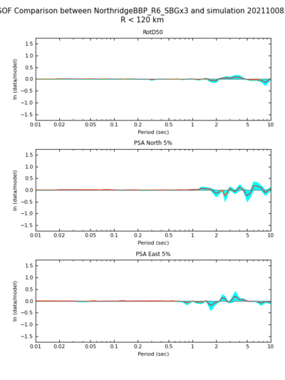
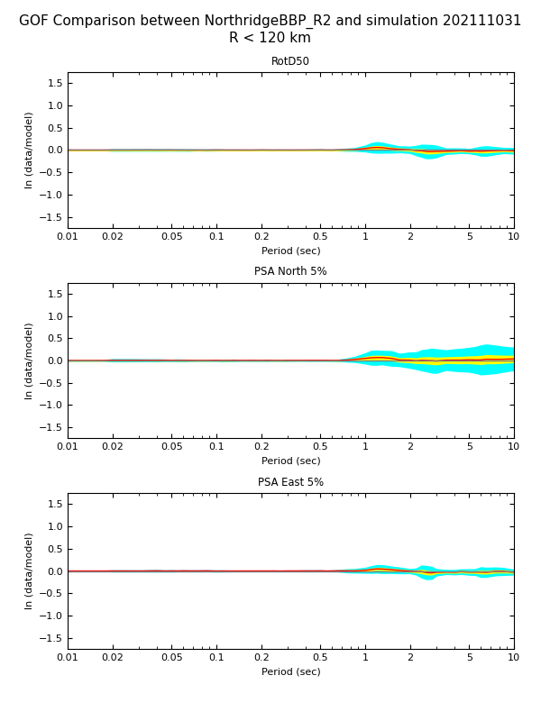
Goodness of fit plots
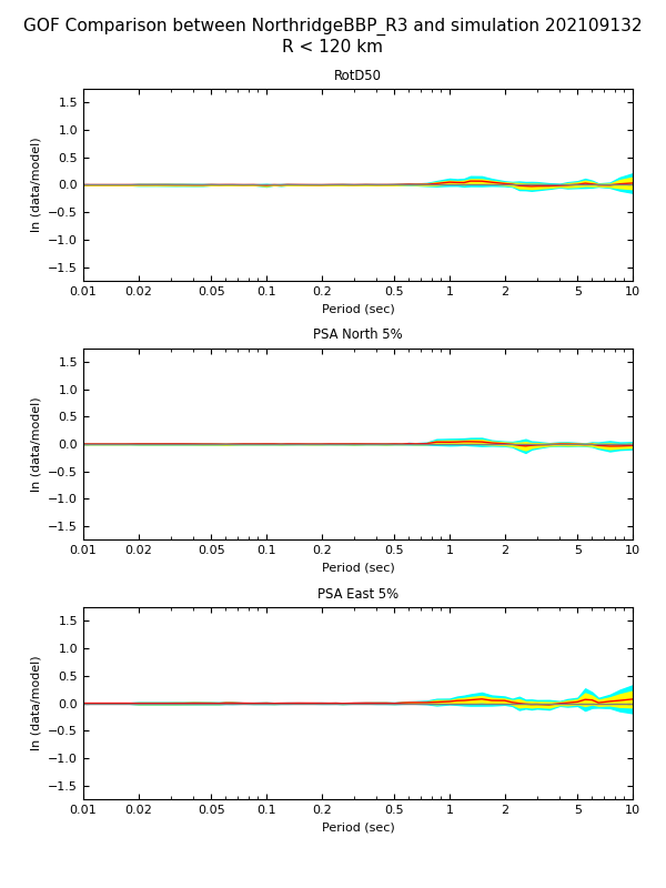
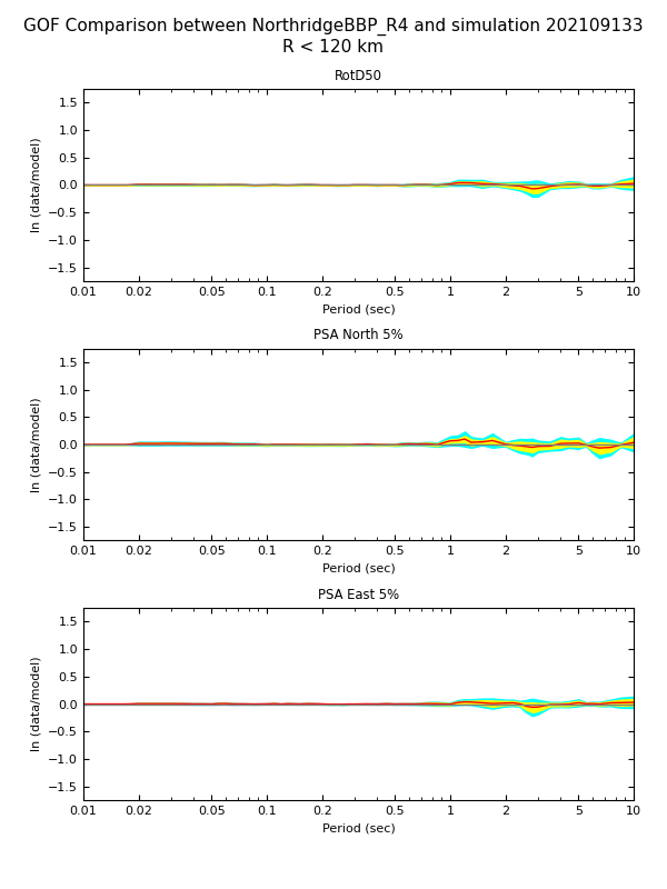
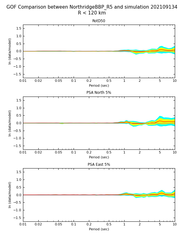
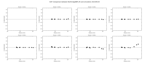
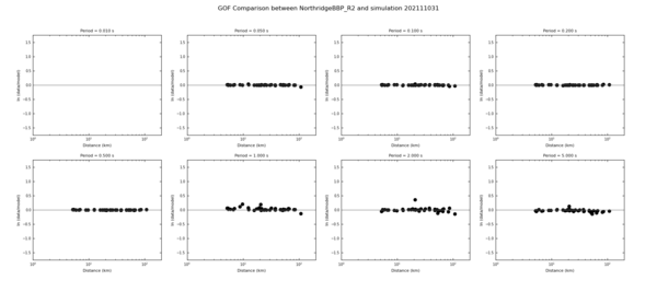
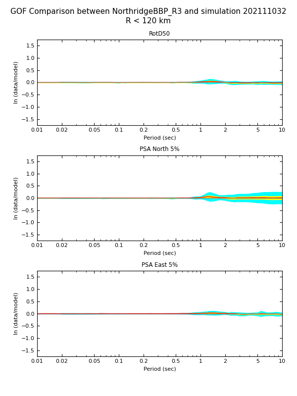
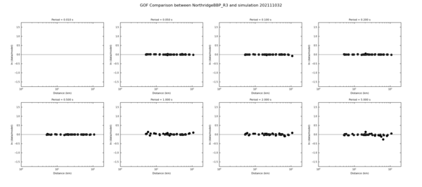
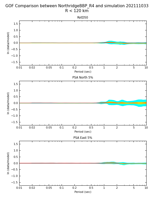
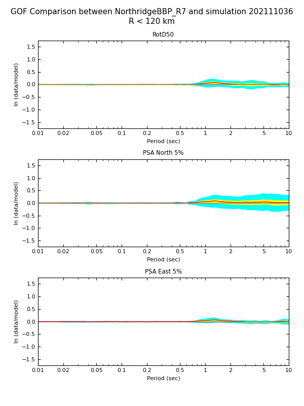
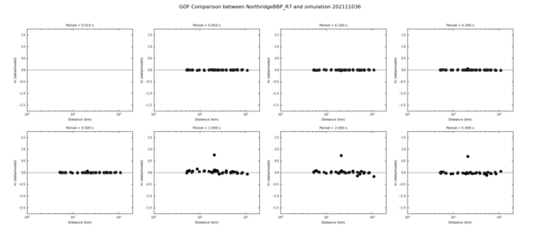
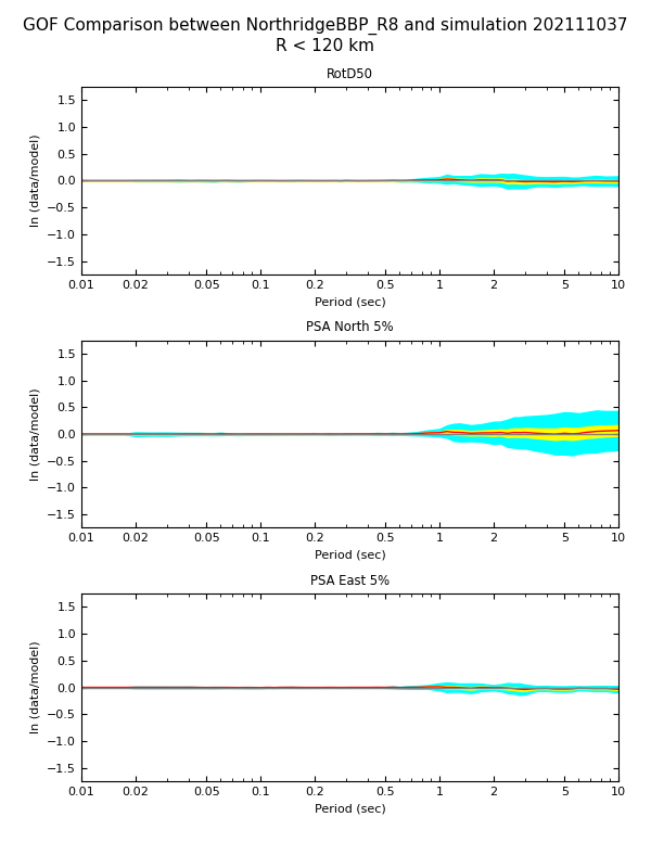
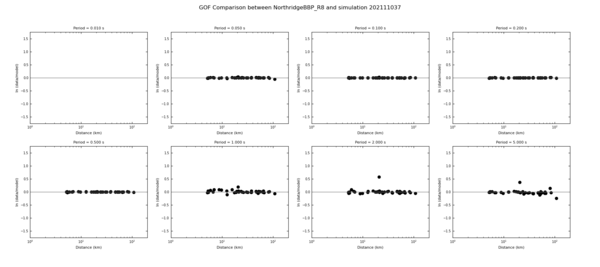
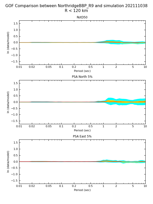
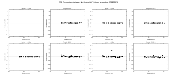
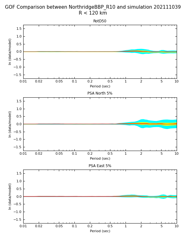
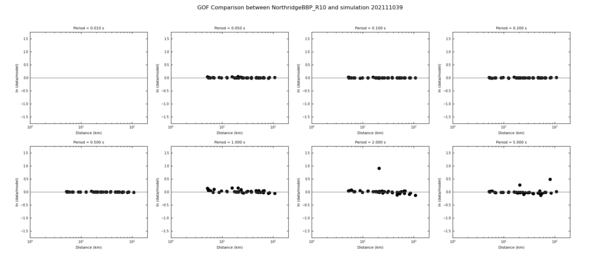
Results for 10 stations, 1 realization
Results for modified interpolation in jbsim3d
GoF for multiple realizations
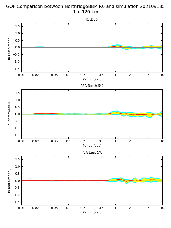
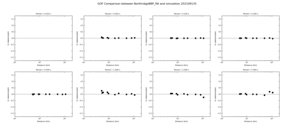
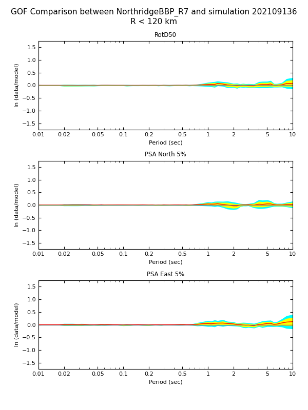
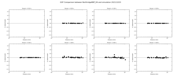
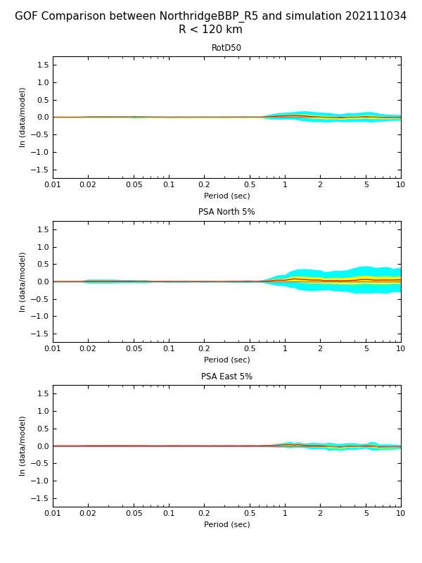
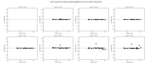
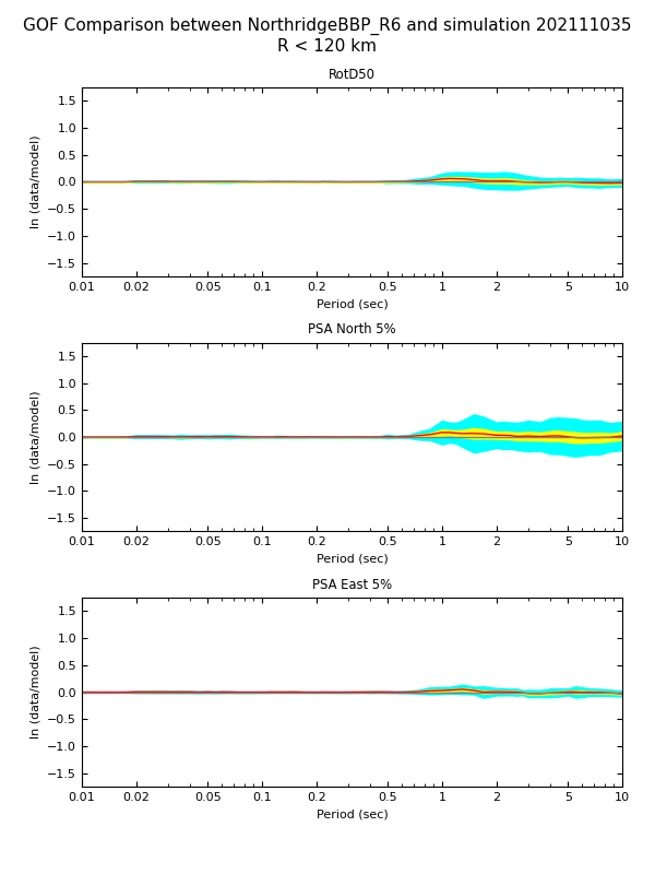
For clarity, here are the steps involved in producing the below plots.
- Generate the 10 realizations by using a random number generator to generate 9 numbers, and create copies of the src file which is used in the BBP validation event, changing only the seed.
- Produce BBP results for each of the 10 sites x 10 realizations. Note that all must be run individually so reproducibility with the random seed isn't an issue.
- Run the BBP workflow generator for 1 site and 1 realization to generate an XML file. This workflow includes SRF generation and site response.
- Using the XML file, replace the path to the station name and the path to the src file.
- Create batch submission scripts which call all 100 BBP workflows.
- Create validation events for each realization.
- Copy over the Northridge validation event data that ships with the BBP.
- Update the data. This includes changing the event name, updating the src file, updating the stl file to filter at the correct frequencies, and stage in the output acceleration data from the BBP runs for the validation event to use as an 'observation'.
- Produce CyberShake results for each of the 10 sites.
- Create a new source in the ERF, in which each realization is a separate rupture of that source.
- Extract the rupture geometry from one of the realizations, to obtain the list of points the SGTs should be saved for.
- Generate a CyberShake volume oriented N/S/E/W which contains the Northridge rupture surface, the site of interest, is 64 km deep, and uses 30 km of padding.
- Generate a velocity mesh using the 24-layer model provided by Rob, which is a post-processed version of the LA Basin 14-layer model included with the BBP.
- Run the original version of the AWP code ('AWP-CS'), using velocity insertion of a source low-pass filtered at 2 Hz, for 30 seconds (unless it's a distance site, in which case we run longer)
- Run the post-processing code for the 10 realizations.
- Run the broadband steps (high-frequency synthesis, low-frequency site response, and merge) for each of the 10 realizations.
- Perform goodness-of-fit, using CyberShake as the simulation and BBP as the reference.
- For each realization:
- Create a temporary directory for the CyberShake results.
- Stage in the CyberShake results for all 10 sites
- Use BBP helper scripts to create a simulation ID and stage the CyberShake results to that directory.
- Run the BBP to generate an XML file which will perform GoF (details at New_BBP_Validation_Package)
- Run using the XML file to generate the GoF comparisons and plots.
- For each realization:
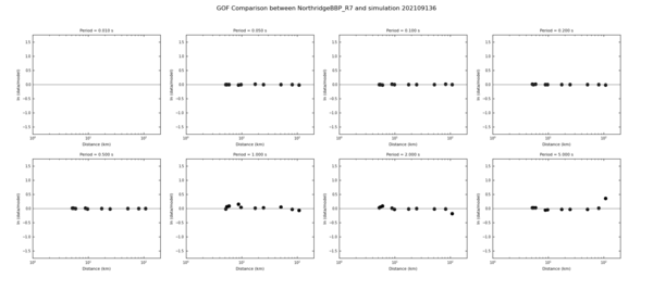
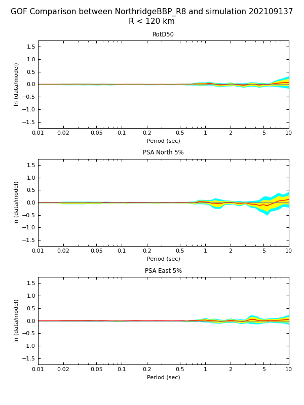
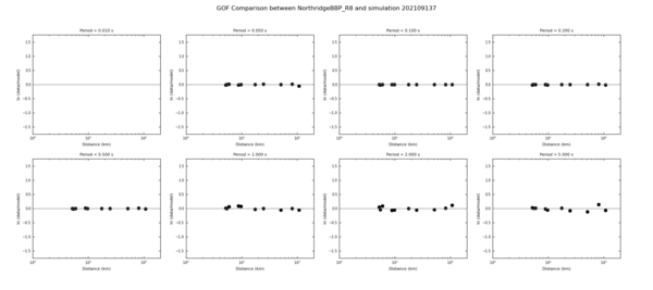
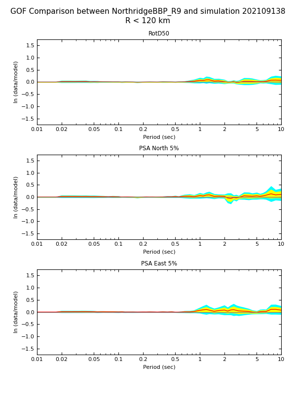
| Realization | GoF plot | Ratio by distance |
|---|---|---|
| 1 | ||
| 2 | ||
| 3 | ||
| 4 | ||
| 5 | ||
| 6 | ||
| 7 | ||
| 8 | ||
| 9 | ||
| 10 |
Combined goodness-of-fit
33m tests
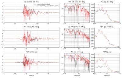
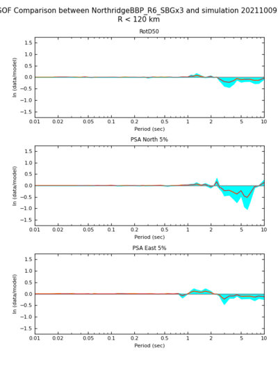
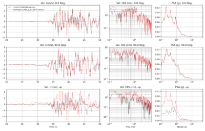
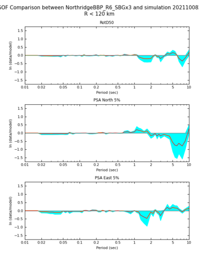
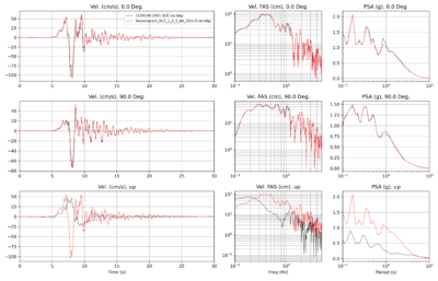
We modified the grid spacing from 100m to 33.333m to see what impact it has on the BBP/CS comparisons. To simplify the comparisons, results here are for 1 Northridge realization, realization 6.
| Site | 100m | 33m |
|---|---|---|
| SCE | ||
| SBG |
Expanded buffer layer tests
When calculating the size of the CyberShake volume, we construct a volume large enough to contain the site and all the fault surfaces, then pad it on all sides by 30 km. We modified the buffer zone to be larger, 50 km.
| Site | 30 km buffer zone | 50 km buffer zone |
|---|---|---|
| SCE | ||
| SBG |
We then performed additional tests, deepening the volume to 80 km, increasing the padding to 60 km, and also increasing the number of grid points in the boundary condition sponge zone from 50 to 80. Below are comparisons with the original results, including GoF for site SBG.
All plots are for Northridge realization 6.
| Site (spacing) | 64 km deep, 30 km padding, 50 point sponge zone | GoF for original configuration | 80 km deep, 60 km padding, 80 point sponge zone | GoF for modified configuration | 80 km deep, 60 km padding, 240 point sponge zone |
|---|---|---|---|---|---|
| SCE (100m) | |||||
| SCE (33m) | |||||
| SBG (100m) | |||||
| SBG (33m) |
We tried SBG for both 100m and 33m, saving the SGTs at the same dt as the BBP (0.1s).
| SBG (100m), sim dt=0.005, SGT dt=0.1 | |
| SBG (33m), sim dt=0.001, SGT dt=0.1 |
Northridge, 38 stations
We ran CyberShake and the BBP for 10 realizations for the 38 distinct stations listed here. Note that 2006-PAC and 2007-PUL are colocated, so we only ran one. Below are goodness-of-fit and scatterplot GOF results.
| Realization | GoF plot | GoF scatterplot |
|---|---|---|
| 2 | ||
| 3 | ||
| 4 | ||
| 5 | ||
| 6 | ||
| 7 | ||
| 8 | ||
| 9 | ||
| 10 |
