Difference between revisions of "Preferred Rupture Directivity in Hazard Curve Computations"
(→Plots: Add San Andreas 100% compute times) |
|||
| Line 121: | Line 121: | ||
Site: University of Southern California (USC) | Site: University of Southern California (USC) | ||
| − | Compute Time: 1min 7s (90p), 48s (100p), 1min 12s (sa25p) | + | Compute Time: 1min 7s (90p), 48s (100p), 1min 12s (sa25p), 1min 23s (sa100p) |
=== ALP 9542 === | === ALP 9542 === | ||
| Line 128: | Line 128: | ||
Site: Antelope (ALP) | Site: Antelope (ALP) | ||
| − | Compute Time: 1min 16s (90p), 1min 12s (sa25p) | + | Compute Time: 1min 16s (90p), 1min 12s (sa25p), 1min 29s (sa100p) |
=== SBSM 9320 === | === SBSM 9320 === | ||
| Line 135: | Line 135: | ||
Site: San Bernardino Strong Motion (SBSM) | Site: San Bernardino Strong Motion (SBSM) | ||
| − | Compute Time: 59s (90p), 1min 1s (100p), 1min 12s (sa25p) | + | Compute Time: 59s (90p), 1min 1s (100p), 1min 12s (sa25p), 1min 24s (sa100p) |
=== SVD 9647 === | === SVD 9647 === | ||
| Line 142: | Line 142: | ||
Site: Seven Oaks Dam (SVD) | Site: Seven Oaks Dam (SVD) | ||
| − | Compute Time: 1min 16s (90p), 1min 13s (sa25p) | + | Compute Time: 1min 16s (90p), 1min 13s (sa25p), 1min 26s (sa100p) |
=== PDE 9663 === | === PDE 9663 === | ||
| Line 149: | Line 149: | ||
Site: Pardee (PDE) | Site: Pardee (PDE) | ||
| − | Compute Time: 1min 21s (90p), 1min 4s (sa25p) | + | Compute Time: 1min 21s (90p), 1min 4s (sa25p), 1min 25s (sa100p) |
Revision as of 16:03, 3 September 2025
This page documents efforts to investigate the impact that preferred rupture directions would have on hazard as calculated with CyberShake ground motions in OpenSHA.
Contents
Research Plan
There is some evidence that some faults have a preferred rupture direction. To investigate the impact this could have on hazard, we'll identify a handful of faults, modify the probabilities of individual rupture variations to favor those at the preferred end of the fault, and generate new hazard products with the modified probabilities. No new ground motions will need to be calculated; we'll use Study 22.12 and 24.8 ground motions.
Below is a flow chart representing the steps involved in performing this work.
Implementation Details
With the UCERF2 ERF used in Study 22.12 and Study 24.8, probabilities are specified at the rupture level -- that is, for a specific fault segment(s) and magnitude. We then divide the probability by the number of rupture variations to get the uniform probability of each rupture variation. For this work, we will create modified rupture variation probabilities and use these to generate a modified hazard curve.
We will add new functionality to the CyberShake-related code in OpenSHA to support this work. OpenSHA has a defined interface to return a list of probabilities for a given source ID and rupture ID. We'll specify the source ID, rupture ID, rupture variation ID, probability in a CSV file which will be passed to OpenSHA. This file will be parsed and used to populate a data structure, which will then be accessed by an implementation of the interface to determine the new probabilities. For any source ID, rupture ID, rupture variation ID combinations not in the file, we'll use the default UCERF2 probabilities. Then the new probabilities will be used to create a hazard curve.
Modifying the HazardCurvePlotter to allow us to input custom probabilities for rupture variations allows us to compare hazard expected for persistent directivity vs random rupture direction. We can prescribe directivity based on topography or physics reasons and see if the signature is drowned out by randomness of the network or if it still stands out.
Unlike the UCERF2 ERF in standard PSHA, CyberShake utilizes an extended ERF that supports rupture variation probabilities. Both include ruptures, but by specifying hypocenter, we're able to support directivity.
In standard OpenSHA, the hierarchy is sources which are fault segments, down to ruptures which are collection of faults. CyberShake extended ERFs add another layer, rupture variations. These identify the place on the fault where the hypocenter is and define a slip-time history.
New Functionality
The existing OpenSHA command-line tool, HazardCurvePlotter, is able to compute hazard curves and plot them to images locally on a system. We’ve added a new parameter, rv-probs-csv, for a Rupture Variation Probabilities Input CSV file.
Passing this file allows a user to specify directivity for specific rupture variations. Previously, all variations had an equal probability, distributed from the probability of the rupture itself. The sum of probabilities of the variations must still sum to the probability of the corresponding rupture.
CSV Files
CSV Structure
The input CSV file should have the following columns.
- Source_ID
- Rupture_ID
- Rup_Var_ID
- Probability
The specified source and rupture acts as a composite key, uniquely identifying a rupture variation. Each rupture at a site is comprised of a set of rupture variations. The CSV file does not need to have an entry for each variation found in the CyberShake database. The remaining unspecified variations are given an equal probability distributed from the difference of the rupture probability and the sum of rupture variation probabilities specified. The formatting, structure, and sum or probabilities are validated in the HazardCurvePlotter.
CSV Generation
To generate the CSV files used for these tests, we created a Python script which takes in a configuration file and outputs a CSV with modified probabilities for selected rupture variations.
The Python script is available here.
Inputs
Here are the CSV files used so far.
- USC_reference_probs.csv : Reference input with same probabilities as fetched from DB for site=USC, run=9306
- USC_mod_probs_Mojave_Coachella.csv : 10% hypocenter responsible modified probabilities for site=USC, run=9306
- USC_mod_probs_Mojave_Coachella_90p.csv : 90% modified probability site=USC, run=9306
- USC_mod_probs_Mojave_Coachella_100p.csv : 100% modified probability site=USC, run=9306
- USC_mod_probs_Moj_Coach_sa25p.csv : 25% modified prob, all San Andreas Events for site=USC, run=9306
- USC_mod_probs_Moj_Coach_sa100p.csv : 100% modified prob, all San Andreas Events for site=USC, run=9306
- ALP_mod_probs_Mojave_Coachella_90p.csv : 90% modified probability site=ALP, run=9542
- ALP_mod_probs_Moj_Coach_sa25p.csv : 25% modified prob, all San Andreas Events for site=ALP, run=9542
- ALP_mod_probs_all_Moj_Coach_100p.csv : 100% modified prob, all San Andreas Events for site=ALP, run=9542
- SBSM_mod_probs_Mojave_Coachella_90p.csv : 90% modified probability site=SBSM, run=9320
- SBSM_mod_probs_Mojave_Coachella_100p.csv : 100% modified probability site=SBSM, run=9320
- SBSM_mod_probs_Moj_Coach_sa25p.csv : 25% modified prob, all San Andreas Events for site=SBSM, run=9320
- SBSM_mod_probs_all_Moj_Coach_100p.csv : 100% modified prob, all San Andreas Events for site=SBSM, run=9320
- SVD_mod_probs_Mojave_Coachella_90p.csv : 90% modified probability site=SVD, run=9647
- SVD_mod_probs_Moj_Coach_sa25p.csv : 25% modified prob, all San Andreas Events for site=SVD, run=9647
- SVD_mod_probs_all_Moj_Coach_100p.csv : 100% modified prob, all San Andreas Events for site=SVD, run=9647
- PDE_mod_probs_Mojave_Coachella_90p.csv : 90% modified probability site=PDE, run=9663
- PDE_mod_probs_Moj_Coach_sa25p.csv : 25% modified prob, all San Andreas Events for site=SVD, run=9647
- PDE_mod_probs_all_Moj_Coach_100p.csv : 100% modified prob, all San Andreas Events for site=SVD, run=9647
Plots
The following plots show curves for the following sites:
- ALP
- USC
- SBSM
- SVD
- PDE
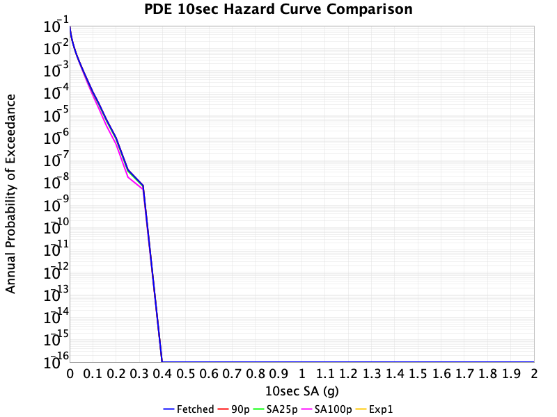
There is a plot for each site of the periods (K) 2, 3, 5, and 10, for a total of 20 plots. Each figure has the following plot lines
- The reference using original probabilities (Ref)
- Where hypocenters are responsible for 90% of the probability (90p)
- USC and SBSM has additional plot line where hypocenters are responsible for 100% (100p)
- 25% probability over All San Andreas Events (sa25p)
- 100% probability over All San Andreas Events (sa100p)
The hazard curve plots were generated using the following bash scripts:
- plot_fetch_curves.sh fetches curves from database
- plot_modified_curves.sh generates curves using input biases
./plot_fetch_curves.sh
./plot_modified_curves.sh modprob/90p csv 90p
./plot_modified_curves.sh modprob/100p csv 100p
./plot_modified_curves.sh modprob/sa25p csv/all_san_andreas sa25p
./plot_modified_curves.sh modprob/sa100p csv/all_san_andreas sa100p
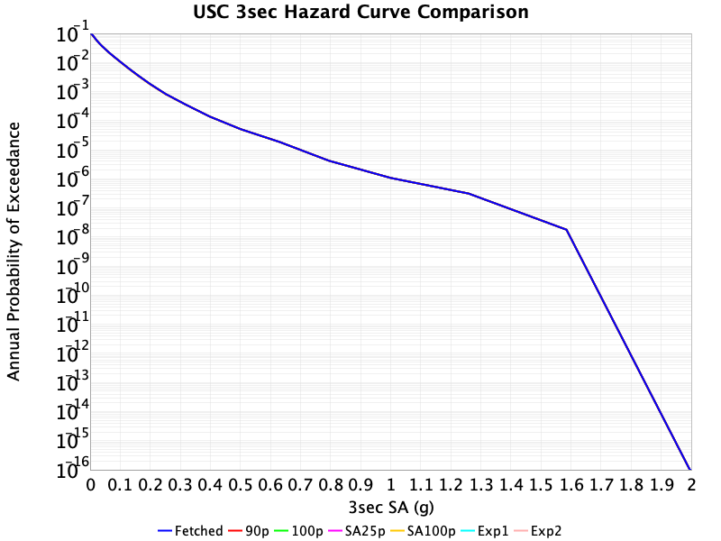
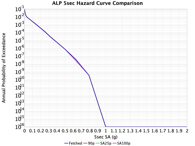
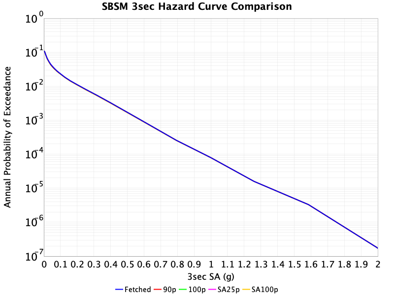
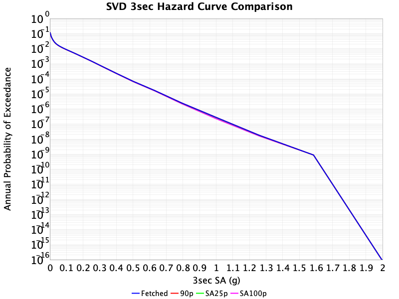
For the 10p, 90p, and 100p plots, the results are identical to the fetched probabilities. When considering all events across the San Andreas, we see significant impact to PDE and ALP, some impact to SVD, and no visible significant impact to SBSM and USC.
For the sake of brevity, we won't show all 20 plots here.
The X,Y data points and all plots generated are available in the Excel spreadsheet : File:Hazard Curve Comparison Plots.xlsx
Comparison plots were made by copying out the TXT X,Y datapoints into Excel. We may expand existing OpenSHA Comparison Plot functionality for this purpose. Currently we're able to compare a new run against results fetched from a database, but not multiple modified plots.
USC 9306
Site: University of Southern California (USC)
Compute Time: 1min 7s (90p), 48s (100p), 1min 12s (sa25p), 1min 23s (sa100p)
ALP 9542
Site: Antelope (ALP)
Compute Time: 1min 16s (90p), 1min 12s (sa25p), 1min 29s (sa100p)
SBSM 9320
Site: San Bernardino Strong Motion (SBSM)
Compute Time: 59s (90p), 1min 1s (100p), 1min 12s (sa25p), 1min 24s (sa100p)
SVD 9647
Site: Seven Oaks Dam (SVD)
Compute Time: 1min 16s (90p), 1min 13s (sa25p), 1min 26s (sa100p)
PDE 9663
Site: Pardee (PDE)
Compute Time: 1min 21s (90p), 1min 4s (sa25p), 1min 25s (sa100p)

