Difference between revisions of "Wills Map"
From SCECpedia
Jump to navigationJump to search| (7 intermediate revisions by 2 users not shown) | |||
| Line 1: | Line 1: | ||
== Wills References == | == Wills References == | ||
| − | *Wills 2015 | + | |
| − | * Wills 2006 - C.J. and Clahan, K.B., [2006], Developing a map of geologically defined site-conditions categories for California: Bull. Seism. | + | * Wills, Christopher & Gutierrez, Carlos & Perez, Ante & Branum, David. (2015). A Next Generation V S 30 Map for California Based on Geology and Topography. Bulletin of the Seismological Society of America. 105. 10.1785/0120150105. |
| − | Soc. Am., Vol. 96 pp. 1483 – 1501 | + | *[https://www.researchgate.net/publication/283670069_A_Next_Generation_V_S_30_Map_for_California_Based_on_Geology_and_Topograpy Wills 2015] |
| + | * Wills 2006 - C.J. and Clahan, K.B., [2006], Developing a map of geologically defined site-conditions categories for California: Bull. Seism. Soc. Am., Vol. 96 pp. 1483 – 1501 | ||
| + | |||
| + | == Description of Wills Digital Map == | ||
| + | <pre> | ||
| + | |||
| + | The supplementary data of the Wills et al. (2015) paper provides the map as a GIS shapfile (http://www.seismosoc.org/Publications/BSSA_html/bssa_105-6/2015105-esupp/index.html). I then rasterized it to a binary floating point file (which similar to the 2006 file, except with floats instead of short ints) using the gdal_rasterize command (http://www.gdal.org/gdal_rasterize.html). The command to rasterize it is: | ||
| + | |||
| + | gdal_rasterize -a Vs30_Mean -tr $RES $RES -l wills_2015_vs30_projected -of EHdr -ot Float32 ./wills_2015_vs30_projected.shp ./raster_$RES.flt | ||
| + | |||
| + | Where $RES is the grid spacing in degrees. | ||
| + | |||
| + | The original and rasterized data is stored here on opensha.usc.edu: | ||
| + | |||
| + | /export/opensha-00/data/siteData/wills_2015 | ||
| + | |||
| + | I suggest you use raster_0.00025.flt, which is rasterized with 0.00025 degree spacing (~25 meters). The raster_0.00025.hdr file contains the necessary coordinates for georeferencing it, but I'll summarize here: | ||
| + | |||
| + | The first location in the file is at: | ||
| + | |||
| + | x/longitude/ULXMAP = -124.406528862058 | ||
| + | y/latitude/ULYMAP = 42.0090923024621 | ||
| + | |||
| + | This is the upper left (northwest) point in the map. | ||
| + | |||
| + | numX/numLon/NCOLS = 41104 | ||
| + | numY/numLat/NROWS = 37900 | ||
| + | |||
| + | Grid spacing (both X and Y): 0.00025 degrees | ||
| + | |||
| + | Data type: 4-byte/32-bit little-endian floating point numbers | ||
| + | |||
| + | Mesh ordering: fast XY, so the first few points are: | ||
| + | |||
| + | Index 0 (at byte 0): -124.406528862058, 42.0090923024621 | ||
| + | Index 1 (at byte 4): -124.406528862058+0.00025, 42.0090923024621 = -124.406278862058, 42.0090923024621 | ||
| + | Index 2 (at byte 8): -124.406528862058+0.0005, 42.0090923024621 = -124.406028862058, 42.0090923024621 | ||
| + | ... | ||
| + | </pre> | ||
| + | |||
| + | |||
| + | == Comparison of Wills Map 2006 versus 2015 == | ||
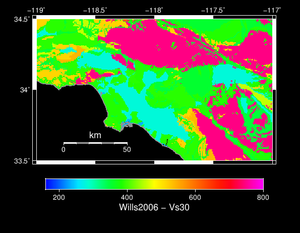
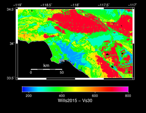
| + | These two wills maps were made from gis files released by the state. | ||
| + | {| | ||
| + | | [[File:wills_2006.png|thumb|300px|Wills Map 2006]] | ||
| + | | [[File:wills_2015.png|thumb|300px|Wills Map 2015]] | ||
| + | |} | ||
| + | |||
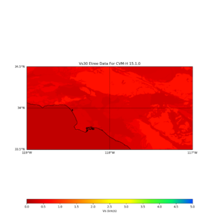
| + | These two wills maps are extracted by ucvm. The etree vs30 values are based on wills 2006, so we expect to see data from above in these maps. | ||
| + | {| | ||
| + | | [[File:Cvmh_nogtl_vs30_etree_map.png|thumb|300px|Vs30 Map based on UCVM Etree for 2006]] | ||
| + | | [[File:wills_2015.png|thumb|300px|Wills Map 2015]] | ||
| + | |} | ||
| + | |||
== grd2etree == | == grd2etree == | ||
| − | + | Background information from | |
https://scec.usc.edu/scecpedia/UCVM_Utah | https://scec.usc.edu/scecpedia/UCVM_Utah | ||
https://github.com/SCECcode/UCVMC/wiki/Manual-Pages | https://github.com/SCECcode/UCVMC/wiki/Manual-Pages | ||
| − | + | Where we worked at in generating the ucvm.e | |
that we are currently using: | that we are currently using: | ||
/home/scec-00/patrices/opt/vs30 | /home/scec-00/patrices/opt/vs30 | ||
| − | + | Created a configure file sample.conf | |
<pre> | <pre> | ||
# grid2etree UCM Map config file | # grid2etree UCM Map config file | ||
| Line 121: | Line 174: | ||
</pre> | </pre> | ||
| − | |||
| − | |||
| − | |||
| − | |||
| − | |||
| − | |||
| − | |||
| − | |||
| − | |||
| − | |||
| − | |||
| − | |||
| − | |||
| − | |||
| − | |||
| − | |||
| − | |||
| − | |||
| − | |||
| − | |||
| − | |||
| − | |||
| − | |||
| − | |||
| − | |||
| − | |||
| − | |||
| − | |||
| − | |||
| − | |||
| − | |||
| − | |||
| − | |||
| − | |||
| − | |||
| − | |||
| − | |||
| − | |||
| − | |||
| − | |||
| − | |||
| − | |||
| − | |||
| − | |||
| − | |||
| − | |||
== Related Entries == | == Related Entries == | ||
*[[CME Project]] | *[[CME Project]] | ||
*[[CyberShake]] | *[[CyberShake]] | ||
Latest revision as of 03:23, 16 April 2020
Contents
Wills References
- Wills, Christopher & Gutierrez, Carlos & Perez, Ante & Branum, David. (2015). A Next Generation V S 30 Map for California Based on Geology and Topography. Bulletin of the Seismological Society of America. 105. 10.1785/0120150105.
- Wills 2015
- Wills 2006 - C.J. and Clahan, K.B., [2006], Developing a map of geologically defined site-conditions categories for California: Bull. Seism. Soc. Am., Vol. 96 pp. 1483 – 1501
Description of Wills Digital Map
The supplementary data of the Wills et al. (2015) paper provides the map as a GIS shapfile (http://www.seismosoc.org/Publications/BSSA_html/bssa_105-6/2015105-esupp/index.html). I then rasterized it to a binary floating point file (which similar to the 2006 file, except with floats instead of short ints) using the gdal_rasterize command (http://www.gdal.org/gdal_rasterize.html). The command to rasterize it is:

gdal_rasterize -a Vs30_Mean -tr $RES $RES -l wills_2015_vs30_projected -of EHdr -ot Float32 ./wills_2015_vs30_projected.shp ./raster_$RES.flt

Where $RES is the grid spacing in degrees.

The original and rasterized data is stored here on opensha.usc.edu:

/export/opensha-00/data/siteData/wills_2015

I suggest you use raster_0.00025.flt, which is rasterized with 0.00025 degree spacing (~25 meters). The raster_0.00025.hdr file contains the necessary coordinates for georeferencing it, but I'll summarize here:

The first location in the file is at:

x/longitude/ULXMAP = -124.406528862058
y/latitude/ULYMAP = 42.0090923024621

This is the upper left (northwest) point in the map.

numX/numLon/NCOLS = 41104
numY/numLat/NROWS = 37900

Grid spacing (both X and Y): 0.00025 degrees

Data type: 4-byte/32-bit little-endian floating point numbers

Mesh ordering: fast XY, so the first few points are:

    Index 0 (at byte 0): -124.406528862058, 42.0090923024621
    Index 1 (at byte 4): -124.406528862058+0.00025, 42.0090923024621 = -124.406278862058, 42.0090923024621
    Index 2 (at byte 8): -124.406528862058+0.0005, 42.0090923024621 = -124.406028862058, 42.0090923024621
    ...
Comparison of Wills Map 2006 versus 2015
These two wills maps were made from gis files released by the state.
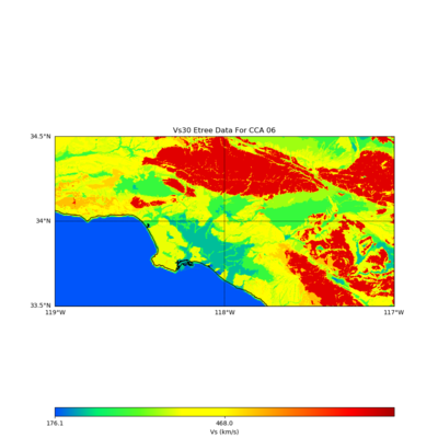
These two wills maps are extracted by ucvm. The etree vs30 values are based on wills 2006, so we expect to see data from above in these maps.
grd2etree
Background information from
 https://scec.usc.edu/scecpedia/UCVM_Utah
 https://github.com/SCECcode/UCVMC/wiki/Manual-Pages
Where we worked at in generating the ucvm.e that we are currently using:
/home/scec-00/patrices/opt/vs30
Created a configure file sample.conf
# grid2etree UCM Map config file

# Domain corners coordinates (degrees):
proj=+proj=aeqd +lat_0=36.0 +lon_0=-120.0 +x_0=0.0 +y_0=0.0
lon_0=-129.75
lat_0=40.75
rot=55.0

# Domain dimensions (meters):
x-size=1800000.0
y-size=900000.0

# Spacing
spacing=250.0

# Etree parameters and info
title=UCVM_Elev_Vs30_Map_Wills_Wald
author=P_Small
date=05/2011
outputfile=ucvm.e

# Grid data directories
elev_hr_dir=/home/scec-00/patrices/opt/ned
elev_lr_dir=/home/scec-00/patrices/opt/bath
vs30_hr_dir=/home/scec-00/patrices/opt/vs30/wills_gridfloat
vs30_lr_dir=/home/scec-00/patrices/opt/vs30/wald_gridfloat
NOTE: the ucvm.e newly recreated is 1.2G but UCVMC's ucvm.e is 683M
command used to generate ucvm.e
./grd2etree -f sample.conf
new ucvm.e
A new ucvm.e is created by replacing the vs30_hr_dir with the rasterized data file from Kevin and update the hdr file to match with what is expected by grd2etree
#BYTEORDER      I
LAYOUT         BIL
nrows          37900
ncols          41104
NBANDS         1
NBITS          32
BANDROWBYTES   164416
TOTALROWBYTES  164416
PIXELTYPE      FLOAT

#ULXMAP         -124.406528862058
#ULYMAP         42.0090923024621
xllcorner         -124.406528862058
yllcorner         32.534092
cellsize          0.00025
NODATA_value  -9999
byteorder     LSBFIRST
XDIM           0.00025
YDIM           0.00025
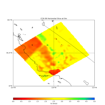
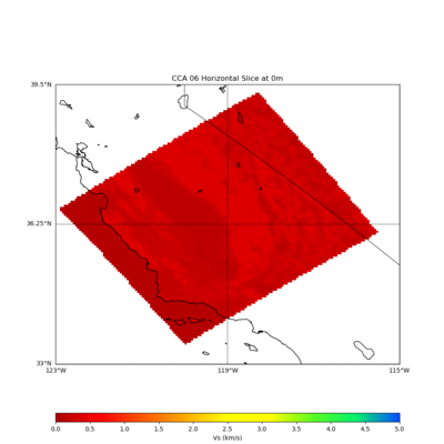
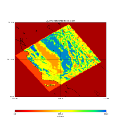
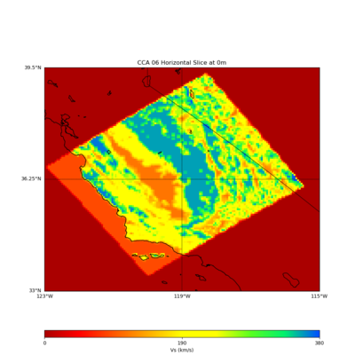
Verify using CCA+GTL
| With fixed scale | ||
|---|---|---|
| With fixed scalebar, | ||
| With variable scalebar, | ||
command used to generate the plots,
./plot_horizontal_slice.py -b 33,-123 -u 39.5,-115 -d vs -c cca -a sd -s 0.05 -e 0 -o cca.png
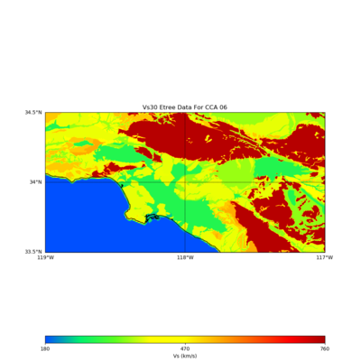
Verify using vs30 etree map
| With variable scale | |
|---|---|
command used to generate the plots,
./plot_vs30_etree_map.py -b 33.5,-119 -u 34.5,-117 -s 0.0005 -c cca -a sd_r -o cca_vs30_etree_new.png
