Difference between revisions of "Study 18.5 Velocity Model Comparisons"
| Line 36: | Line 36: | ||
/** Brocher 2005 scaling polynomial coefficient 10^5 */ | /** Brocher 2005 scaling polynomial coefficient 10^5 */ | ||
double p5; | double p5; | ||
| + | |||
| + | defined like this: | ||
| + | |||
| + | # Density scaling parameters | ||
| + | p5 = -0.0024189659303912917 | ||
| + | p4 = 0.015600987888334450 | ||
| + | p3 = 0.051962399479341816 | ||
| + | p2 = -0.51231936640441489 | ||
| + | p1 = 1.2550758337054457 | ||
| + | p0 = 1.2948318548300342 | ||
| + | |||
| + | |||
</pre> | </pre> | ||
Revision as of 07:19, 24 May 2018
Contents
Consensus CVM for CyberShake Study 18.5
Based on initial simulations and CVM plot evaluations, we expect to build the CyberShake NorCal Study 18.5 by tiling CVM's in this order USGS Bay Area model (cencal), CCA06 with Ely Geotechnical Layer (cca), CVM-S4.26.M01 (cvmsi). Smoothing will be done on the mesh along horizontal interfaces for a distance of 20km on each side. The smoothing is done using a method that will be described here. Plots of the resulting models are listed below:
Algorithm for calculating density
CVM-S4.26 returns density based on Vs values using the following relationship:
/**
 * Calculates the density based off of Vs. Based on Nafe-Drake scaling relationship.
 *
 * @param vs The Vs value off which to scale.
 * @return Density, in g/m^3.
 */
double calculate_density(double vs) {
        double retVal;
        vs = vs / 1000;
        retVal = configuration->p0 + configuration->p1 * vs + configuration->p2 * pow(vs, 2) +
                         configuration->p3 * pow(vs, 3) + configuration->p4 * pow(vs, 4) + configuration->p5 * pow(vs, 5);
        retVal = retVal * 1000;
        return retVal;
}
These configuration values are based on:
	/** Brocher 2005 scaling polynomial coefficient 10^0 */
	double p0;
	/** Brocher 2005 scaling polynomial coefficient 10^1 */
	double p1;
	/** Brocher 2005 scaling polynomial coefficient 10^2 */
	double p2;
	/** Brocher 2005 scaling polynomial coefficient 10^3 */
	double p3;
	/** Brocher 2005 scaling polynomial coefficient 10^4 */
	double p4;
	/** Brocher 2005 scaling polynomial coefficient 10^5 */
	double p5;

defined like this:

# Density scaling parameters
p5 = -0.0024189659303912917
p4 = 0.015600987888334450
p3 = 0.051962399479341816
p2 = -0.51231936640441489
p1 = 1.2550758337054457
p0 = 1.2948318548300342
Initial CVM Version
For Study 18.5, the first velocity model we examined used the following order of precedence:
- USGS Bay Area model
- CCA-06
- CVM-S4.26.M01 which include a 1D background model
We will apply a minimum Vs of 500 m/s. We will smooth to a distance of 10 km either side of a velocity model interface. A KML file showing the model regions is available here.
We had originally planned to query them in the order 1) USGS Bay Area; 2) CVM-S4.26.M01; 3) CCA-06; 4) 1D background; but upon inspection of the cross-sections, CCA-06 seems to capture the Great Valley basins better than CVM-S4.26, leading to better agreement with the southern edge of the USGS Bay Area model. We are investigating adding the Ely GTL to the CCA-06 model to compensate for the lack of low-velocity, near-surface structure in CCA-06, since the tomographic inversion was performed at 900 m/s.
An alternative velocity model, under consideration for this simulation is based on tiling the models in the following order:
- USGS Bay Area model
- CCA-06 with Ely GTL
- CVM-S4.26 with Ely GTL
- BBP 1D model
Forward simulations
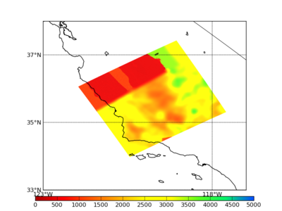
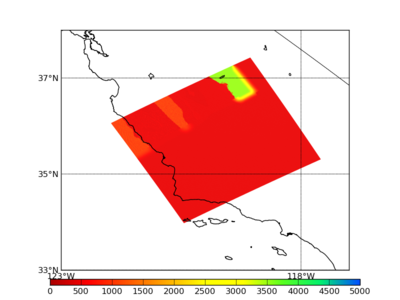
To check the smoothing region, we performed forward simulations near the USGS/CCA-06 boundary, in a volume 270 x 300 x 50 km. The corners of the region are:
-120.5,34,0
-121.93426,36.12917
-118.98101,37.41772
-117.60821,35.25771
For our first test, we selected the CyberShake event ERF ID 36, source ID 60, rupture ID 3, rupture variation 13, a south-to-north M6.95 on the Cholame segment of the San Andreas. We ran with a minimum Vs of 500 m/s, dt=0.005, nt=20000, so 100 sec of simulation time. A visualization of the results is available here; the USGS Bay Area region is in green, and the CCA-06 region is in red. Note that the USGS region has a GTL but the CCA region does not.
For our second test, we selected an individual point in the above CyberShake event and simulated a point source about 20 km SW of the model interface, with the same simulation parameters (minimum Vs of 500 m/s, dt=0.005, nt=20000, so 100 sec of simulation time). A visualization is available here; the USGS Bay Area region is in green, and the CCA-06 region is in red. Note that the USGS region has a GTL but the CCA region does not.
We added the Ely GTL to the CCA-06 model for this region and reran the point-source simulation (with additional filtering). A visualization is available here.
Below are plots comparing the surface without and with the Ely GTL on CCA-06.
Since we saw some refraction effects with the 10 km smoothing, we also tried running with 20 km smoothing, which shows reduced refraction effects. A visualization is available here: [1]
Finally, we did a finite fault simulation across the model interface. We ran ERF 36, source 81, rupture 3, a M7.05 on the San Andreas, the Parkfield and Cholame segments, using the 20 km smoothing. A visualization is available here.
Alternative Velocity Model Plots
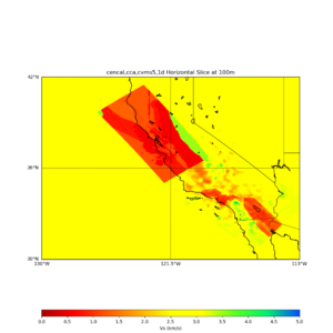
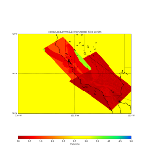
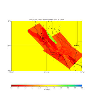
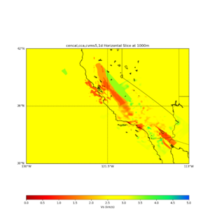
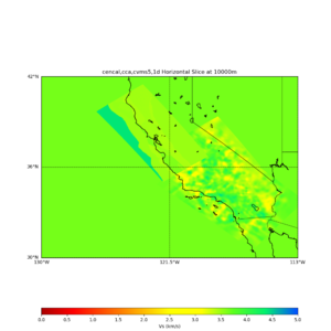
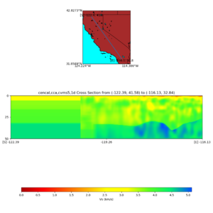
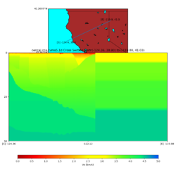
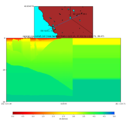
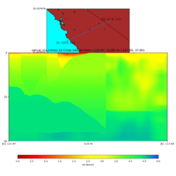
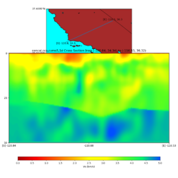
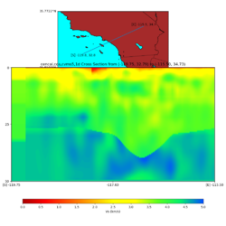
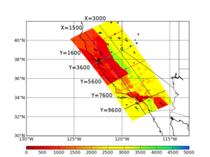
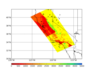
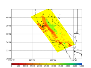
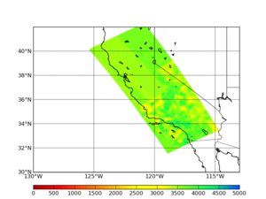
We have updated the CyberShake 18.5 velocity model to tile USGS Bay Area, CCA06, and CVM-S4.26, and a 1D background model. Also we have added the Ely GTL to the models. Then, we extracted horizontal cross-sections at 0 km, 0.1 km, 1 km, and 10 km. The 0 km cross-section also indicates the vertical cross-section locations. The following plots represent a proposed Northern California Velocity Model. There is no smoothing between models in these plots. Smoothing will be done to the final selected collection of CVMs.Thes plots were created using an updated version of the UCVM Software,which is available on a development branch in the ucvmc github repository.
The tiling order of velocity models in these plots is:
Science Name (ucvmc abbreviation):
- USGS Bay Area Model (cencal)
- CCA06 (cca)
- CVM-S4.26 (cvms5)
- Modified Hadley Kanamori 1D (1d)
Tiled without adding Ely-Jordan GTL to CCA06 or CVM-S4.26
Tiled with Ely-Jordan Vs30-based GTL added to CCA06, and CVM-S4.26
Tiled with Ely-Jordan Vs30-based GTL added to CCA06 and CVM-S4.26
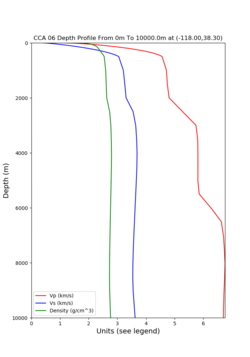
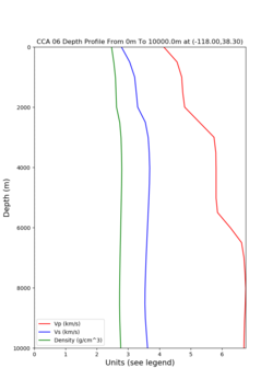
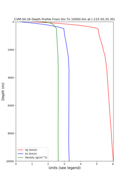
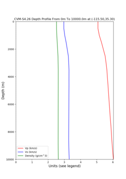
Depth profiles of 2 selected points:
- Point in CCA06 Model (38.3 -118.0 ):
- Point in CVM-S4.26 (35.3 -115.5) :
Original Vs cross-sections
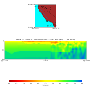
We have extracted horizontal cross-sections at 0 km, 0.1 km, 1 km, and 10 km. The 0 km cross-section also indicates the vertical cross-section locations.
We extracted vertical cross-sections along 5 cuts parallel to the x-axis:
- Y index=1600: (38.929900, -124.363400) to (41.030000, -119.880200)
- Y index=3600: (37.413200, -123.140900) to (39.470700, -118.713500)
- Y index=5600: (35.884300, -121.967300) to (37.900400, -117.598200)
- Y index=7600: (34.344500, -120.838200) to (36.319900, -116.529600)
- Y index=9600: (32.794700, -119.750000) to (34.730300, -115.503600)
The southeast edge is on the left side of the plots.
and 2 cuts parallel to the y-axis:
- X index=1500: (40.866500, -123.900300) to (32.207800, -117.529700)
- X index=3000: (41.579900, -122.388500) to (32.844200, -116.127900)
The northwestern edge is on the left of the plots.
