Difference between revisions of "Broadband CyberShake Validation"
| Line 423: | Line 423: | ||
== Landers == | == Landers == | ||
| + | |||
| + | === BBP === | ||
| + | |||
| + | |||
| + | |||
| + | === CyberShake === | ||
Revision as of 20:05, 7 December 2022
This page follows on CyberShake BBP Verification, moving from 1D comparisons to 3D CyberShake comparisons with both the BBP and observations.
Contents
Process
These are the steps involved in comparing CyberShake and BBP results to observations for a verification event.
BBP
- Create a working directory.
- Create an src_files directory inside it.
- Copy the src file from the BBP validation directory into the src_files directory.
- Copy the station list into the working directory.
- Run run_bbp.py with the '--expert -g' arguments to create an XML file description of the run. Instead of using the defaults for the validation event, point to the station list file in the working directory and the src file in the src_files directory. Include the GP GOF, but not FAS.
- Create 64 realizations by copying over the initial src file and changing the random seed.
- Create 64 directories, one for each source.
- Copy over the setup_lsf_files.sh script. Edit the xml_file_timestamp value to the XML file generated with the run_bbp.py script. You may also need to edit the find/replace lines to reflect the correct path to the .src and .srf files.
- Edit the run_bbp_src.lsf script. Change the xml_file_timestamp, the sim_id, and the name of the event.
- Run setup_lsf_files.sh, which will copy over the run_bbp_src.lsf script into every realization directory and make the needed changes for that realization index.
- Submit all 64 src_*/run_bbp_src*.lsf files.
- Once all 64 run successfully, make a purple_plot/Sims directory, and logs, indata, tmpdata, and outdata directories inside it.
- Edit stage_purple_plot.sh to have the right sim_id.
- Run stage_purple_plot.sh .
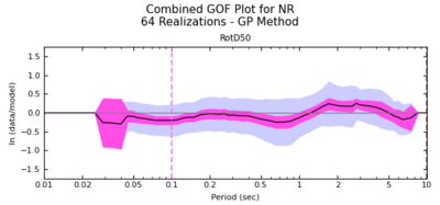
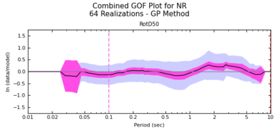
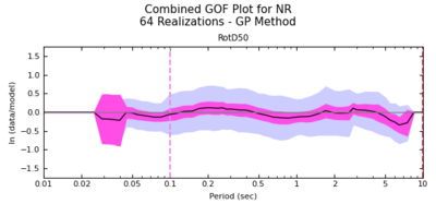
- Run utils/batch/combine_gof_gen.py -d purple_plot -o . -c gp
- Examine the .png file produced to make sure it looks OK.
CyberShake
- Create a working directory.
- Copy the src_files directory from the Broadband validation run directory.
- Copy in the *.stl file from the BBP for this validation event.
- Create site_list.txt, with one CyberShake site per line.
- From another CyberShake validation directory, copy in the following scripts:
- import.lsf
- prep.lsf
- prep_stat.sh
- rename.py
- run_gof.sh
- stage_purple_plot.sh
- run_cs_src0.lsf
- Create a .tgz file on shock with the seismograms for all the stations and all the events.
- Unzip this .tgz file into the working directory.
- Submit prep.lsf. This will copy the seismograms from the station directories into the src directories, and then process them into BBP-friendly format.
- Edit rename.py, and then run it to rename the seismograms to include the full BBP site names.
- Edit import.lsf to use the correct Run ID prefix and src_id, then submit it. This script will import the seismograms into BBP working directories, so that the BBP can run GoF on them.
- Run the BBP to create an XML file which includes running the GoF. To do this, run
run_bbp.py --expert -g
When prompted, select- 'validation simulation'
- the validation simulation created in the first part from the list
- 'GP'
- no custom source
- yes rupture generator
- custom list
- point to list in the working directory
- yes site response
- yes velocity seismogram plots
- yes acceleration seismogram plots
- no GMPE comparisons
- yes goodness-of-fit
- 'GP'
- no additional metrics
Copy the created XML file into the working directory.
- Edit run_cs_src0.lsf and set SIM_ID_PREFIX, DIR_NAME, and XML_PREFIX to the correct values for this event.
- Edit run_gof.sh to set DIR_NAME and XML_PREFIX to the same values.
- Run run_gof.sh, which will submit a job to calculate GoF for each of the 64 realizations.
- Create the directory purple_plot/Sims. Inside there, create 4 directories: logs, indata, tmpdata, and outdata.
- Edit stage_purple_plot.sh to use the correct sim id.
- Create the directory purple_plot_output.
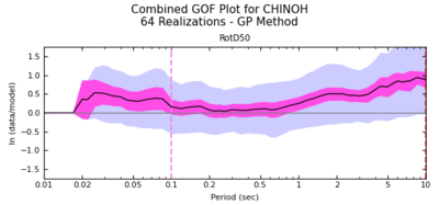
- Run bbp/utils/batch/combine_gof_gen.py -d purple_plot -o purple_plot_output -c gp to produce a purple plot, combining the GoF results from all stations and events.
- Run bbp/utils/batch/compare_bbp_runs.py -d purple_plot -o purple_plot_output/ -c gp to generate the bias values.
Northridge
1D BBP comparisons
We calculated 64 realizations for Northridge for these 38 stations.
Some of the differences between the 1D BBP and 3D CyberShake results can be attributed to differences in site response, which is calculated based on the reference velocity ('vref') and the vs30 of the site. A spreadsheet with vref and Vs30 for both the BBP and CyberShake is available File:BBP v CyberShake Northridge vs30.xls
V1 (2/14/22)
Initially, we used vref=500 for both the high-frequency and low-frequency site response. However, this is incorrect; vref for the low-frequency should vary depending on the properties of the 3D velocity mesh.
V2 (2/25/22)
We continued to use vref=500 for the high-frequency site response. For the low-frequency site response, we are now using the same vref we used in Study 15.12:
vref_LF_eff = Vs30 * [ VsD5H / Vs5H ]
Vs30 = 30 / Sum (1/(Vs sampled from [0.5,29.5] in 1 meter increments))
H = grid spacing
Vs5H = travel time averaged Vs, computed from the CVM in 1 meter increments down to a depth of 5*H
VsD5H = discrete travel time averaged Vs computed from 3D velocity mesh used in the SGT calculation over the upper 5 grid points
So, for H=100m Vs5H would be:
Vs500 = 500 / ( Sum ( 1 / Vs sampled from [0.5,499.5] in 1 meter increments ))
And then VsD5H is given by:
VsD500 = 5/{ 0.5/Vs(Z=0m) + 1/Vs(Z=100m) + 1/Vs(Z=200m) + 1/Vs(Z=300m) + 1/Vs(Z=400m) + 0.5/Vs(Z=500m) }
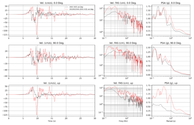
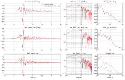
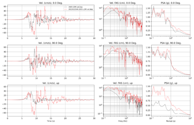
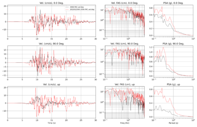
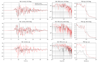
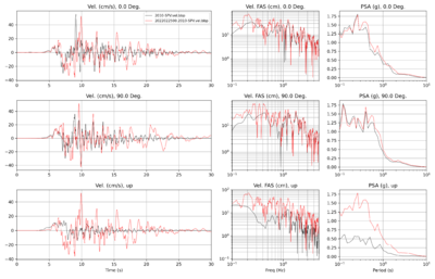
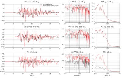
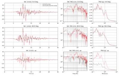
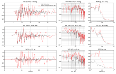
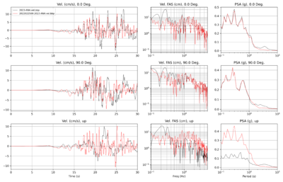
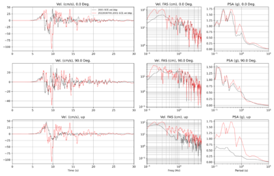
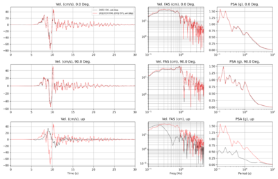
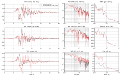
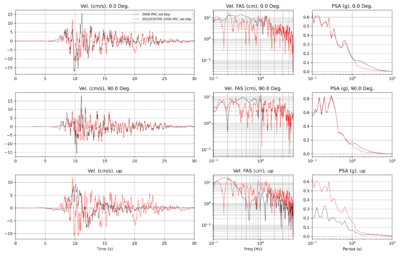
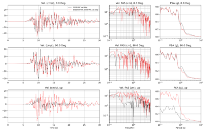
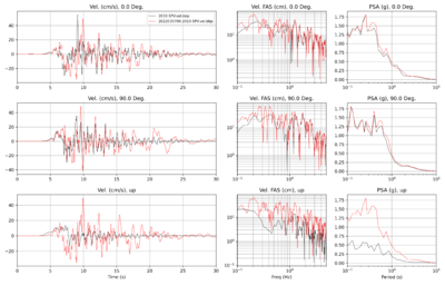
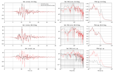
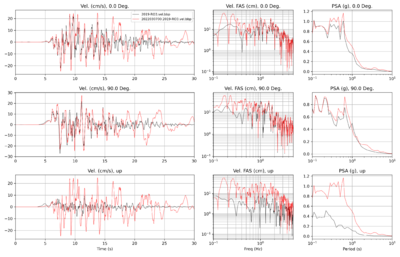
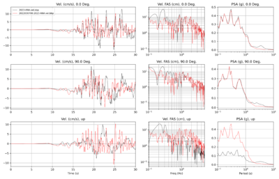
Below are the ts_process plots for a subset of 10 stations, comparing the 3D CyberShake with 1D BBP results.
| Site | TS Process plot |
|---|---|
| SCE | |
| SYL | |
| LDM | |
| PAC | |
| PKC | |
| SPV | |
| WON | |
| KAT | |
| RO3 | |
| ANA |
V3 (3/2/22)
Next, we recalculated the CyberShake results for 10 sites, using the BBP vs30 values for both the low-frequency and high-frequency elements. Note that the vref low-frequency value for CyberShake is still being derived from the velocity model.
| Site | TS Process plot |
|---|---|
| SCE | |
| SYL | |
| LDM | |
| PAC | |
| PKC | |
| SPV | |
| WON | |
| KAT | |
| RO3 | |
| ANA |
Observational Comparisons
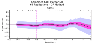
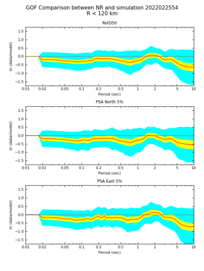
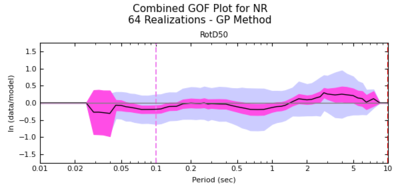
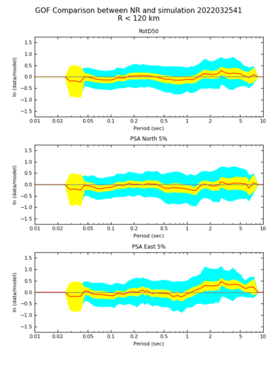
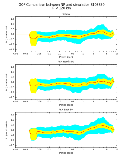
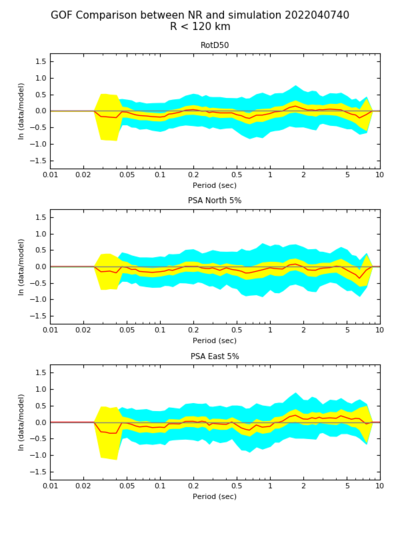
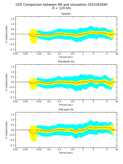
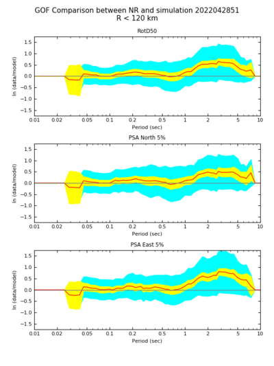
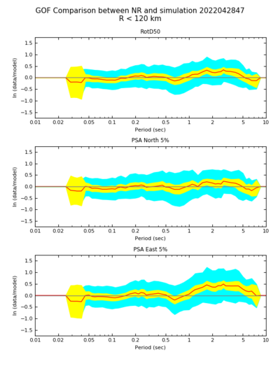
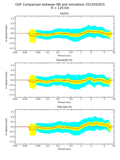
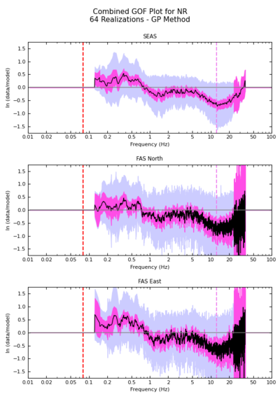
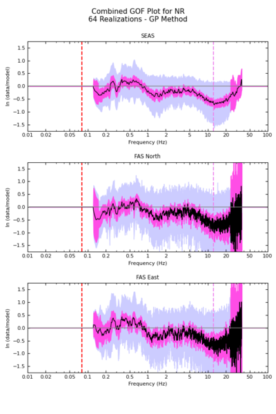
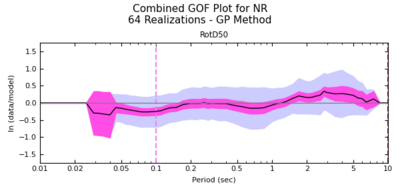
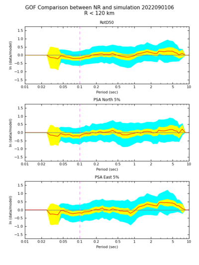
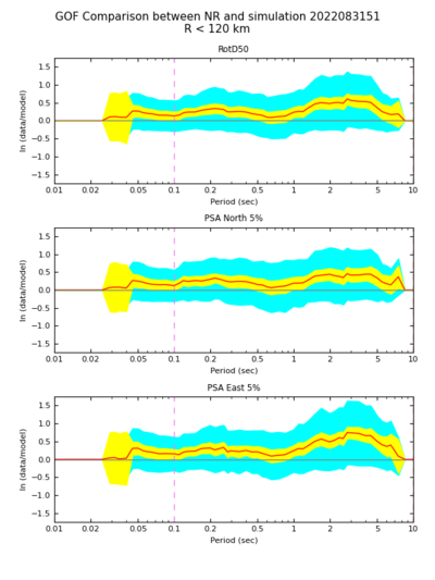
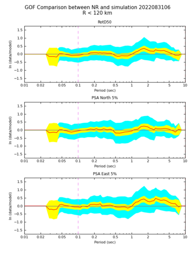
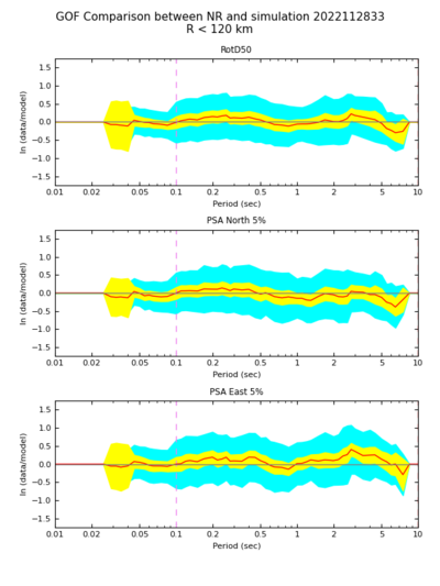
We calculated goodness-of-fit results for both Broadband CyberShake and the BBP against observations for Northridge, using the 64 realizations and 38 stations.
TS process plots comparing the 3 results are available here: v1 ts process plots.
Broadband Platform
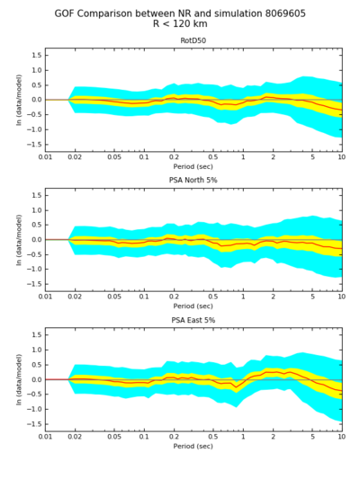
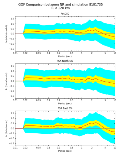
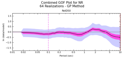
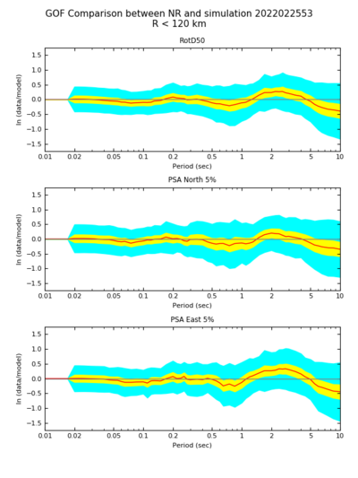
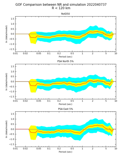
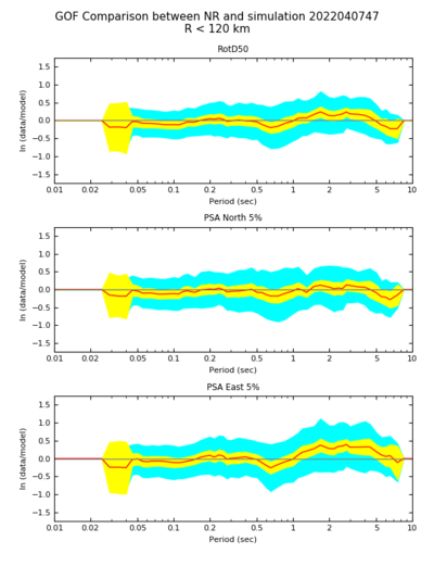
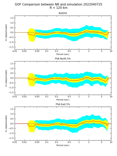
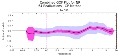
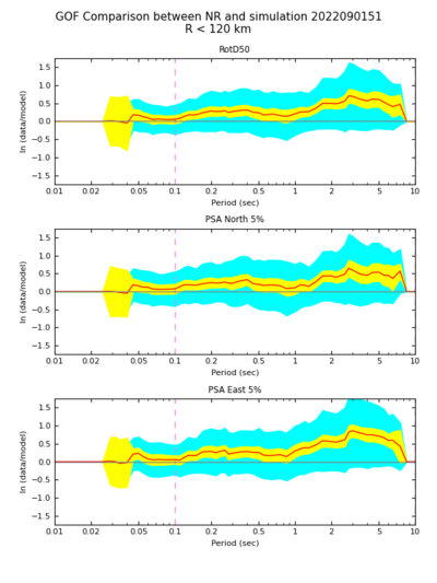
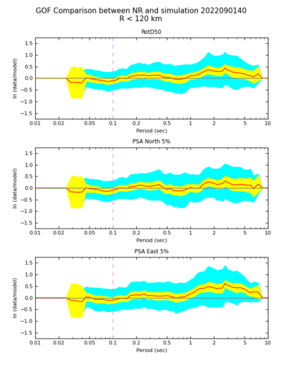
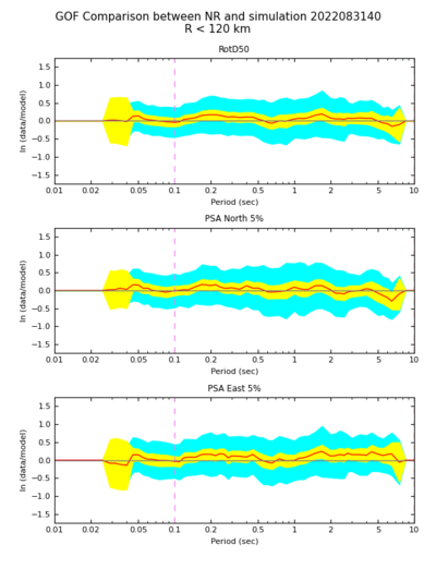
| Overall GoF | GoF, best realization (#7) | GoF, worse realization (#15) |
|---|---|---|
CyberShake v4_8
| Overall GoF | GoF, best realization (#53) | GoF, worse realization (#54) |
|---|---|---|
Broadband Platform, updated frequency bands
We realized that our GoF comparisons were run using hard-coded frequency bands of [0.05, 50] Hz. This was correct when doing CS-to-BBP comparisons, but not correct when using observations. We updated the frequency bands and reran the GoF.
| Overall GoF | GoF, best BBP realization (#47) | GoF, worst BBP realization (#25) | GoF, best CS realization (#40) | GoF, worst CS realization (#37) |
|---|---|---|---|---|
CyberShake v4_8, updated frequency bands
As above, reran the GoF.
| Overall GoF | GoF, best CS realization (#40) | GoF, worst CS realization (#37) | GoF, best BBP realization (#47) | GoF, worst BBP realization (#25) |
|---|---|---|---|---|
CyberShake v4_28, BBP Vs30
We recalculated the CyberShake GoF results, using the BBP Vs30 values.
| Overall GoF | GoF, best CS realization (#40) | GoF, worst CS realization (#51) | GoF, best BBP realization (#47) | GoF, worst BBP realization (#25) |
|---|---|---|---|---|
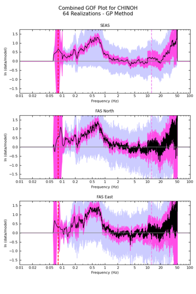
BBP, FAS
CyberShake v4_7, FAS
Observational Comparisons, BBP v22.4
We repeated the comparisons, using BBP v22.4 for both the 1D BBP and 3D CyberShake calculations.
BBP
| Overall GoF | GoF, best BBP realization (#6) | GoF, worst BBP realization (#51) | GoF, best CS realization (#40) | GoF, worst CS realization (#51) |
|---|---|---|---|---|
CyberShake
| Overall GoF | GoF, best CS realization (#40) | GoF, worst CS realization (#51) | GoF, best BBP realization (#6) | GoF, worst BBP realization (#51) |
|---|---|---|---|---|
CyberShake, updated velocity model
| Overall GoF | GoF, best CS realization (#33) | GoF, worst CS realization (#51) |
|---|---|---|
Chino Hills
For our second event, we selected Chino Hills.
Sites
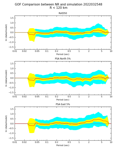
The BBP validation event for Chino Hills has 40 stations. A KML file with the stations is available here.
BBP
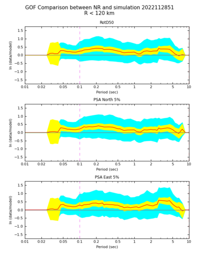
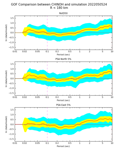
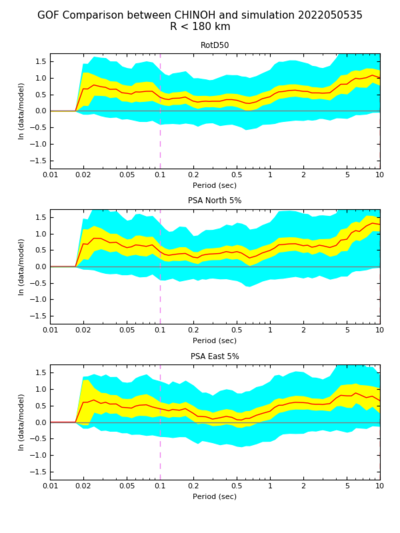
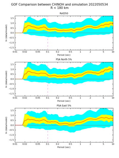
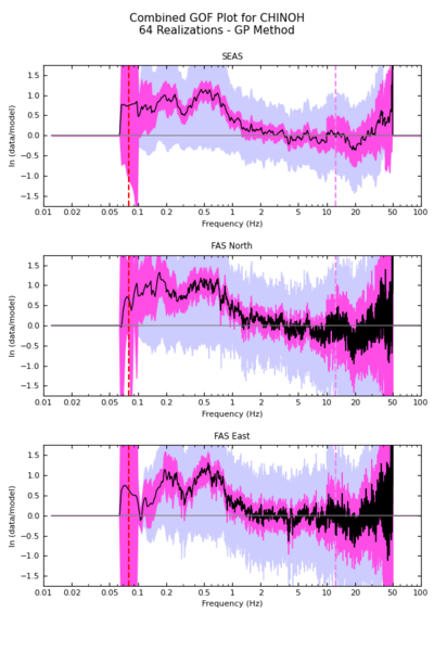
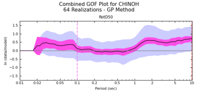
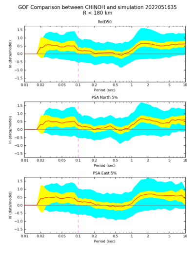
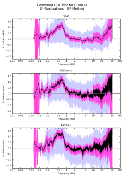
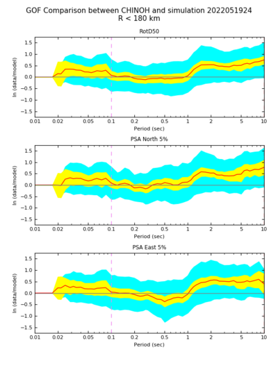
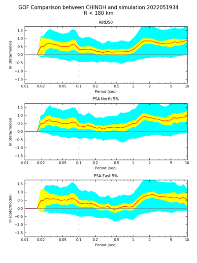
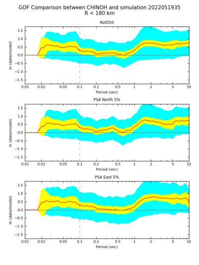
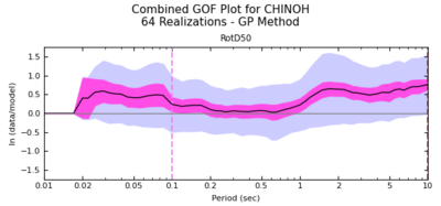
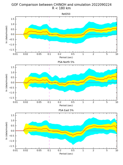
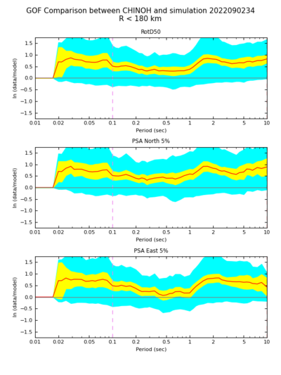
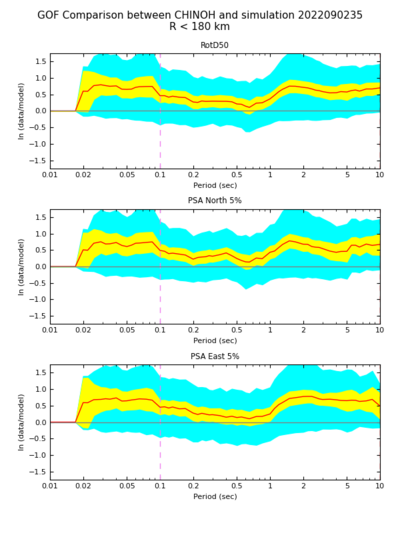
| Overall GoF | GoF, best realization (#24) | GoF, worst realization (#35) | GoF, worst CS realization (#34) |
|---|---|---|---|
CyberShake
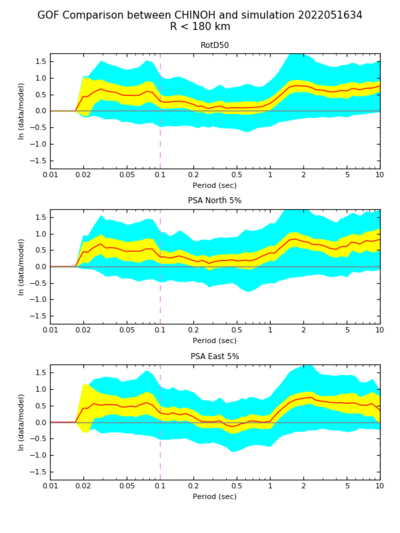
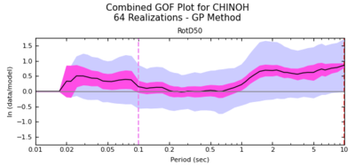
| Overall GoF | GoF, best realization (#24) | GoF, worst realization (#34) | GoF, worst BBP realization (#35) |
|---|---|---|---|
CyberShake, BBP Vs30 values
| Overall GoF | GoF, best realization (#24) | GoF, worst realization (#34) | GoF, worst BBP realization (#35) |
|---|---|---|---|
CyberShake, BBP v22.4
| Overall GoF | GoF, best realization (#24) | GoF, worst realization (#34) | GoF, best BBP realization (#24) | GoF, worst BBP realization (#35) |
|---|---|---|---|---|
CyberShake, BBP v22.4, BBP Vs30
Whittier
Our third event is Whittier.
Sites
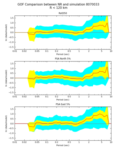
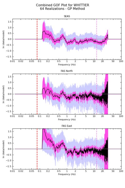
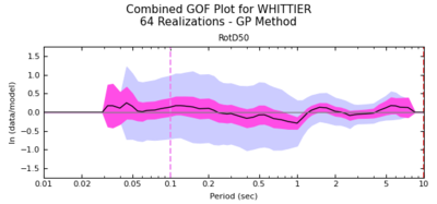
The BBP validation event for Whittier has 39 stations, one of which is a duplicate. A KML file with the 38 stations used in these tests is available here.
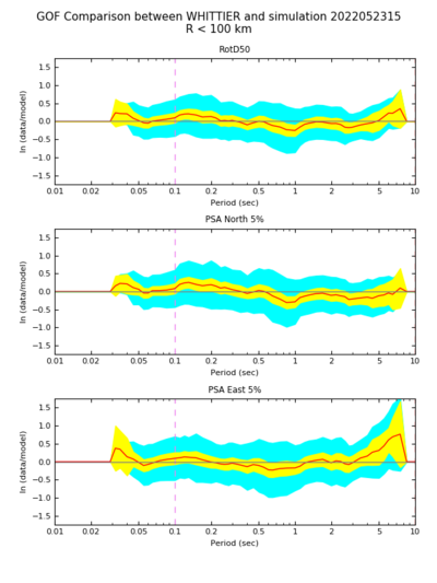
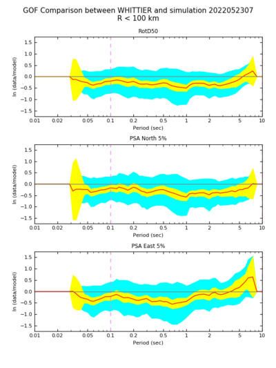
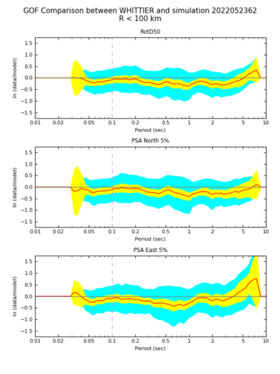
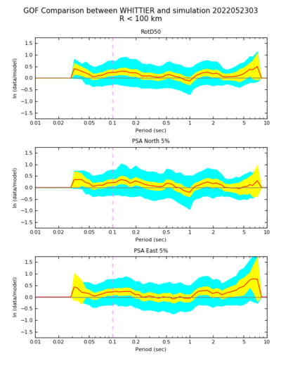
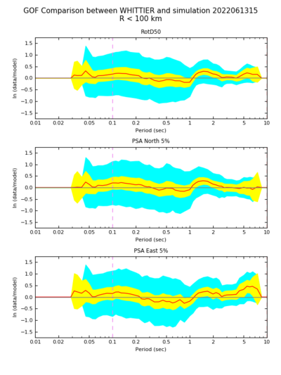
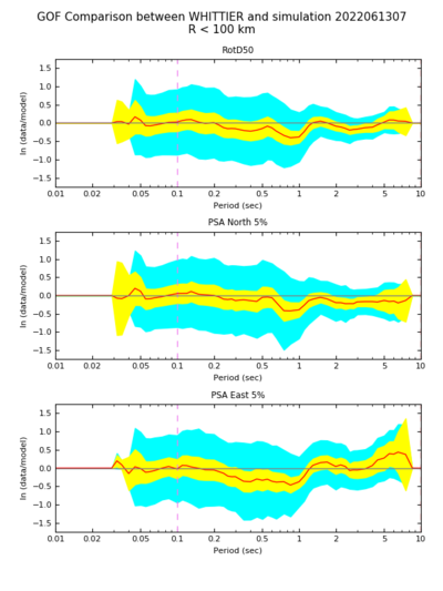
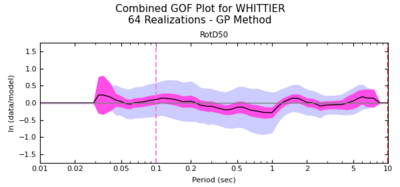
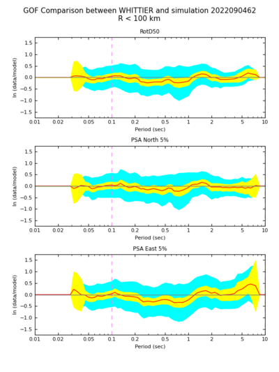
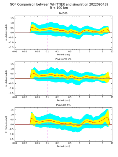
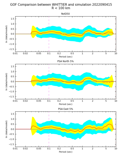
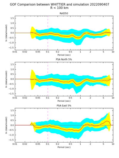
BBP
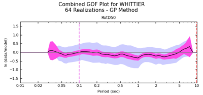
| Overall GoF | GoF, best realization (#15) | GoF, worst realization (#7) | GoF, best CS realization (#62) | GoF, worst CS realization (#3) |
|---|---|---|---|---|
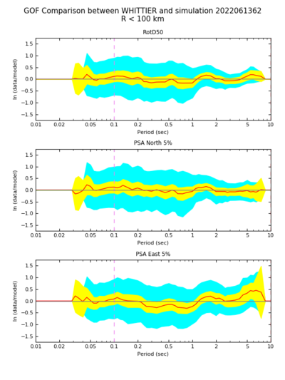
CyberShake
These results are incomplete, without 2 of the stations (VER and PMN).
| Overall GoF | GoF, best realization (#62) | GoF, worst realization (#3) | GoF, best BBP realization (#15) | GoF, worst BBP realization (#7) |
|---|---|---|---|---|
CyberShake, BBP Vs30 values
| Overall GoF | GoF, best realization | GoF, worst realization | GoF, best BBP realization | GoF, worst BBP realization |
|---|---|---|---|---|
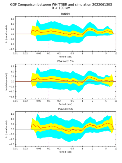
CyberShake, BBP v22.4
| Overall GoF | GoF, best realization (#62) | GoF, worst realization (#39) | GoF, best BBP realization (#15) | GoF, worst BBP realization (#7) |
|---|---|---|---|---|
