CyberShake Tapered Hypocenter Implementation
Motivation
CyberShake Study 15.4 uses the Graves and Pitarka (2015) rupture generator with a uniform hypocenter distribution, including multiple rows of hypocenters down dip. Thus far we have weighted all CyberShake rupture variations equally. This page documents efforts to modify these hypocenter probabilties, reducing probabilities of hypocenters at the edges of the fault. This is similar to the weighted random calculation done by Graves and Pitarka (2015) when random hypocenters are enabled.
Tapered Hypocenter PDF
We apply a taper as follows:
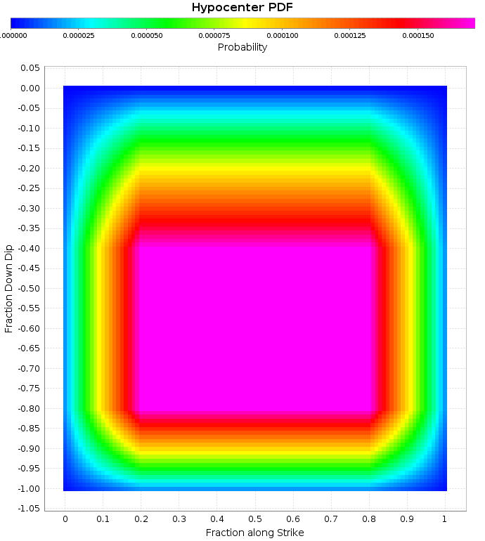
Taper the first and last 20% along strike, starting with 10% weight at each edge. Taper the top (shallowest) 40% and bottom (deepest) 20% of the fault, starting with 1% weight at the top and 10% on the bottom.
Here is the resultant probability density function (PDF)
We calculate the hypocenter location for each rupture variation with srf_gethypo. This returns the grid point with the earliest slip in the SRF file, which is not necessarily identical to the input hypocenter location in the rupture generator.
We then calculate fractional distance along strike and down depth for each hypocenter and apply the taper. Here are the tapered hypocenters for two ruptures with identical surfaces but different magnitudes for a SAF Mojave S source (Source 90, Ruptures 0 & 3). I chose this source as it is fairly planar with 90 degree dip. I then plot the hypocenters (colored circles) as a function of distance along strike and distance down dip. I also plot the input hypocenters (gray circles) on the regular grid before they are perturbed. You can see how even the "uniform" hypocenters show a relatively large amount of scatter:
| Source 90, Rup 0 | 
|
|---|---|
| Source 90, Rup 3 | 
|
| Source 90, Rup 6 | 
|
Hazard Curves
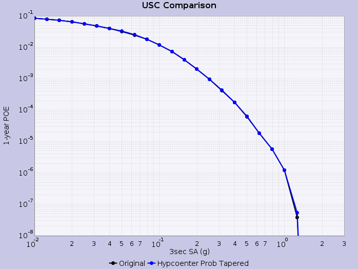
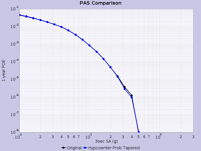
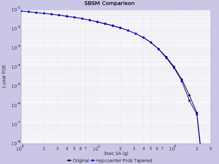
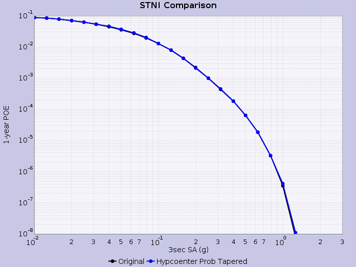
We then calculate hazard curves in OpenSHA, where rupture variations are weighted by the aforementioned tapered hypocenter PDF. We calculate the tapered probability for each rupture variation, rescale such that the total probability summed across all rupture variations is equal to the input probability (UCERF2) for the rupture, and construct an empirical intensity measure exceedence distribution for each rupture using these weighted rupture variation probabilities.
Hazard curves are shown below for select sites applying this methodology:
Hazard Maps
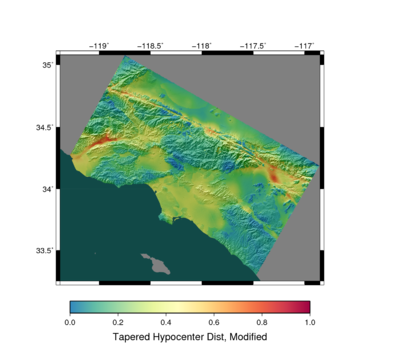
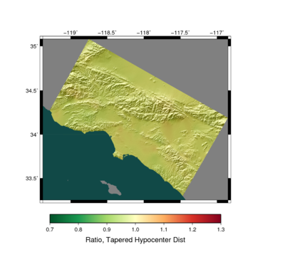
We can also calculate full hazard maps with this tapered hypocenter PDF. Results are shown below, demonstrating the impact is small at the 2% in 50 year hazard level.
