Seismtools
This page describes the seismogram processing package called Seismtools, originally created by Ricardo Taborda's research group at the University of Memphis. This package was forked from its original location at ASEIS/seismtools and developed at SCEC's SCECcode/seismtools GitHub repository. Modifications and improvements to the code were contributed back to ASEIS' original repository. Here's a link to SCEC's forked seismtools repository:
Here's a brief description of some of the software components included in the seismtools repository:
- process_sdc.py - Processes Southern California Data Center ASCII files and generates Hercules format files
- process.py - Processes Strong Motion Center V1/V2 files and generates Hercules format files
- gof.py - Front end for producing GOF results, reads Hercules files, processes their signals, calculates scores and produces table
- gof_data_sim.py - Functions used by the gof.py script to process seismograms
- compare.py - Creates displacement, velocity, and acceleration comparison plots between two Hercules-formated files
- s_compare.py - Processes two Hercules files, and plots only velocity time series, FAS, and Response Spectra
- seism.py - Common structures (e.g. seismic record, station, etc)
- stools.py - Processing functions that can be used by other codes
The basic workflow for processing observation files and generating comparison plots is:
- Run process_sdc.py and/or process.py to convert seismograms to Hercules format
- Run gof.py code to process the observation and synthetic seismogram files, generating processed files and a table containing gof scores
- Run s_compare.py and/or compare.py to generate plots using the processed seismogram files generated by the gof.py stage above
Both processing observation seismograms scripts can be used to convert files to Hercules format in batch mode by taking a directory as input:
$ process_sdc.py /Users/shima/Desktop/Python_Steps/raw_data/ascii/
== Enter event ID (optional):
== Enter network code (optional):
== Enter station ID (optional):
== Enter sample rate and data type representation (optional):
== Enter name of the directory to store outputs: ascii
or
$ process.py  /Users/shima/Desktop/Python_Steps/raw_data/v/
== Enter name of the directory to store outputs: v
Then, users should run the gof.py tool in order to process the Hercules format seismograms and generate rotated/aligned/filtered seismograms:
$ gof.py /Users/shima/Desktop/Python_Steps/filelist
== Enter name of 1st input directory: /Users/shima/Desktop/Python_Steps/her
== Enter name of 2nd input directory: /Users/shima/Desktop/Python_Steps/sim
== Enter name of the directory to store outputs: /Users/shima/Desktop/Python_Steps/gof
== Enter name of scores file: scores.txt
== Enter name of matrics file: metrics.txt
== Enter the sequence of sample rates: 0.1 0.25 0.5 1
== Enter the maximum frequence for decimation: 2
== Enter common dt of two signals: 0.1
== Enter azimuth for rotation (optional): 39.9
== Enter the earthquake start time (#:#:#.#): 11:50:11.916
== Enter the simulation leading time (sec): 2
== Enter the X and Y coordinates of epicenter: 130962.750445 72713.652041
In case we want to run only two signals, we can use:
$ gof.py /Users/shima/Desktop/Python_Steps/her/CI.ALP.BH.her /Users/shima/Desktop/Python_Steps/sim/station.498
== Enter name of the directory to store outputs: out
== Enter name of scores file: scores.txt
== Enter name of matrics file: metrics.txt
== Enter the sequence of sample rates: 0.1 0.25 0.5 1
== Enter the maximum frequence for decimation: 2
== Enter common dt of two signals: 0.1
== Enter azimuth for rotation (optional): 39.9
== Enter the earthquake start time (#:#:#.#): 11:50:11.916
== Enter the simulation leading time (sec): 2
.....
Do you want to print the processed signals [y] or [n]: y
Once the processing stage is completed, users can generate plots using the following commands:
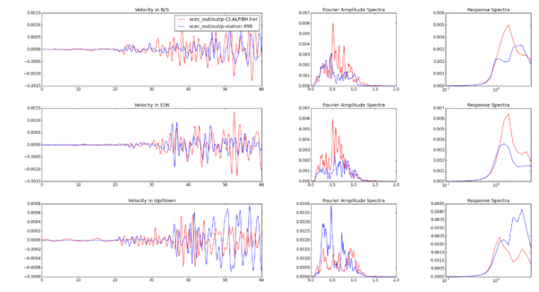
$ compare.py /Users/shima/Desktop/Python_Steps/out/p-CI.ALP.BH.her /Users/shima/Desktop/Python_Steps/out/p-station.498
== Enter T-min for ploting: 0
== Enter T-max for ploting: 60
== Enter F-min for ploting: 0
== Enter F-max for ploting: 2
== Do you want to filter the data (y/n): n
== Enter tmin for Response: 0
== Enter tmax for Response: 5
== Do you want to cut the signal (y/n): n
and:
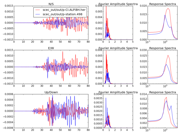
$ s_compare.py /Users/shima/Desktop/Python_Steps/out/p-CI.ALP.BH.her /Users/shima/Desktop/Python_Steps/out/p-station.498
== Enter T-min for ploting: 0
== Enter T-max for ploting: 80
== Enter F-min for ploting: 0
== Enter F-max for ploting: 5
== Do you want to filter the data (y/n): y
== Enter fmin for FAS: 0.5
== Enter fmax for FAS: 2
== Enter tmin for Response: 0
== Enter tmax for Response: 5
== Do you want to cut the signal (y/n): n
La Habra Observations versus Hercules Syhthetics
2016-06-23
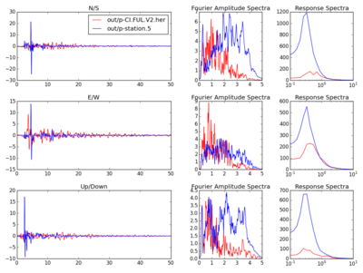
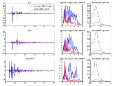
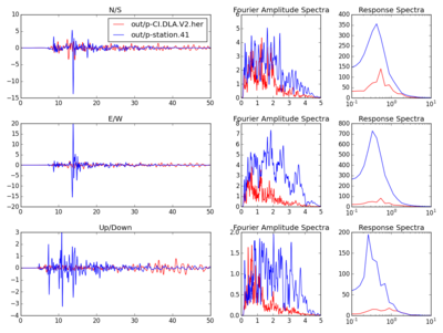
The plots below show La Habra observations compared to synthetic seismograms generated by Hercules for the following stations: FUL, BRE, DLA. The following parameters were used:
- gof.py
== Enter the sequence of sample rates: 0.15 0.25 0.5 1 2 4
== Enter the maximum frequence for decimation: 5
== Enter common dt of two signals: 0.025
== Enter azimuth for rotation (optional): 39.9
== Enter the earthquake start time (#:#:#.#): 4:9:42.97
== Enter the simulation leading time (sec): 0
- s_compare:
== Enter T-min for ploting: 0
== Enter T-max for ploting: 50
== Enter F-min for ploting: 0
== Enter F-max for ploting: 5
== Do you want to filter the data (y/n): n
== Enter tmin for Response: 0
== Enter tmax for Response: 10
== Do you want to cut the signal (y/n): n
- FUL
- BRE
- DLA
Adding BBP File Format Compatibility
The seismtools package has been modified so that it is compatible with time series in BBP format. The process_smc.py script was modified so that the user is asked what format to output seismograms. In the case of the BBP file format, 3 BBP files are output for each input observation file (one containing each of displacement, velocity, and acceleration).
Here's a sample BBP file (shortened) produced by process_smc.py:
# Station: CI_FUL
#    time= 3/29/14,4:9:36.10 UTC
#     lon= 117.923W
#     lat= 33.872N
#   units= m/s
#
# Data fields are TAB-separated
# Column 1: Time (s)
# Column 2: N/S component ground velocity (m/s) (+ is 000)
# Column 3: E/W component ground velocity (m/s) (+ is 090)
# Column 4: U/D component ground velocity (m/s) (+ is upward)
#
0.0000000   9.027200000e-03   -3.251600000e-03    -5.246600000e-03
0.0100000   9.067900000e-03   -3.256500000e-03    -5.257700000e-03
0.0200000   9.108600000e-03   -3.261100000e-03    -5.268600000e-03
0.0300000   9.149300000e-03   -3.265700000e-03    -5.279400000e-03
0.0400000   9.190000000e-03   -3.270200000e-03    -5.290200000e-03
0.0500000   9.230700000e-03   -3.274700000e-03    -5.300700000e-03
0.0600000   9.271600000e-03   -3.279000000e-03    -5.311200000e-03
