CyberShake Study 17.3
CyberShake Study 16.9 is a computational study to calculate 2 CyberShake hazard models - one with a 1D velocity model, one with a 3D - at 1 Hz in a new region, CyberShake Central California. We will use the GPU implementation of AWP-ODC-SGT, the Graves & Pitarka (2014) rupture variations with 200m spacing and uniform hypocenters, and the UCERF2 ERF. The SGT and post-processing calculations will both be run on both NCSA Blue Waters and OLCF Titan.
Contents
Status
Currently we are in the planning stages and hope to begin the study in January 2017.
Science Goals
The science goals for Study 16.9 are:
- Expand CyberShake to include Central California sites.
- Create CyberShake models using both a Central California 1D velocity model and a 3D model (CCA-06).
- Calculate hazard curves for PG&E pumping stations.
Technical Goals
The technical goals for Study 16.9 are:
- Run end-to-end CyberShake workflows on Titan, including post-processing.
- Show that the database migration improved database performance.
Sites
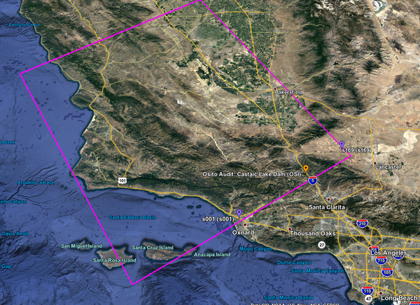
We will run a total of 438 sites as part of Study 16.9. A KML file of these sites, along with the Central and Southern California boxes, is available here (with names) or here (without names).
We created a Central California CyberShake box, defined here.
We have identified a list of 408 sites which fall within the box and outside of the CyberShake Southern California box. These include:
- 310 sites on a 10 km grid
- 54 CISN broadband or PG&E stations, decimated so they are at least 5 km apart, and no closer than 2 km from another station.
- 30 cities used by the USGS in locating earthquakes
- 4 PG&E pumping stations
- 6 historic Spanish missions
- 4 OBS stations
In addition, we will include 30 sites which overlap with the Southern California box (24 10 km grid, 5 5 km grid, 1 SCSN), enabling direct comparison of results.
We will prioritize the pumping stations and the overlapping sites.
Velocity Models
We are planning to use 2 velocity models in Study 16.9. We will enforce a Vs minimum of 900 m/s, a minimum Vp of 1600 m/s, and a minimum rho of 1600 kg/m^3.
- CCA-06, a 3D model created via tomographic inversion by En-Jui Lee. This model has no GTL. Our order of preference will be:
- CCA-06
- CVM-S4.26
- SCEC background 1D model
- CCA-1D, a 1D model created by averaging CCA-06 throughout the Central California region.
We will run the 1D and 3D model concurrently.
Verification
Since we are moving to a new region, we calculated GMPE maps for this region, available here: Central California GMPE Maps
As part of our verification work, we plan to do runs using both the 1D and 3D model for the following 3 sites in the overlapping region:
- s001
- OSI
- s169
Once we are comfortable with those results, we will do runs with the 1D and 3D models for the following sites:
- Bakersfield (-119.018711,35.373292), Wald Vs30 = 206
- Santa Barbara (-119.698189,34.420831), Wald Vs30 = 332
- Parkfield (-120.432800,35.899700), Wald Vs30 = 438
Study 15.4 Verification
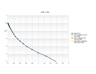
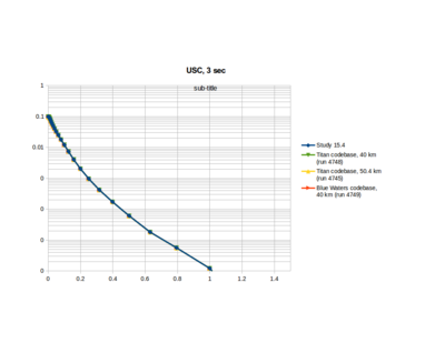
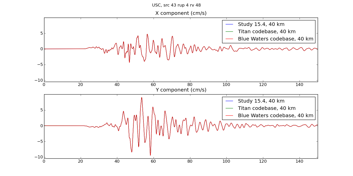
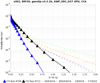
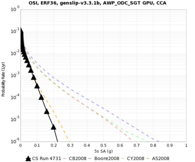
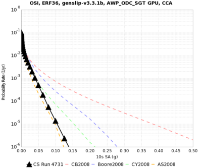
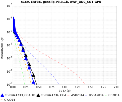
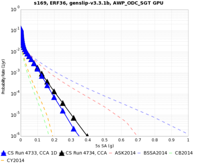
We ran the USC site through the Study 16.9 code base on both Blue Waters and Titan with the Study 15.4 parameters. Hazard curves are below, and very closely match:
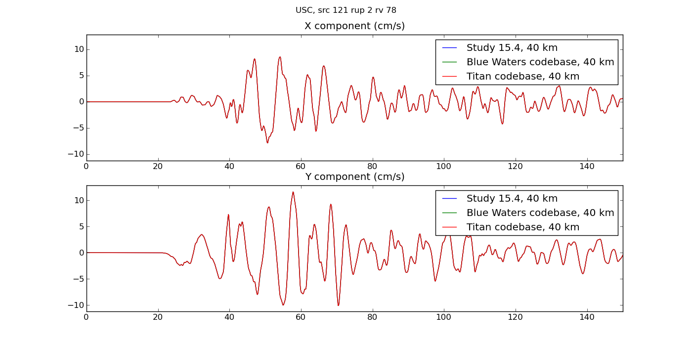
Plots of the seismograms show excellent agreement:
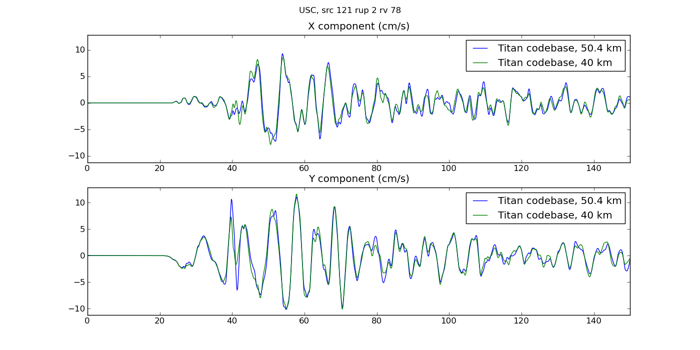
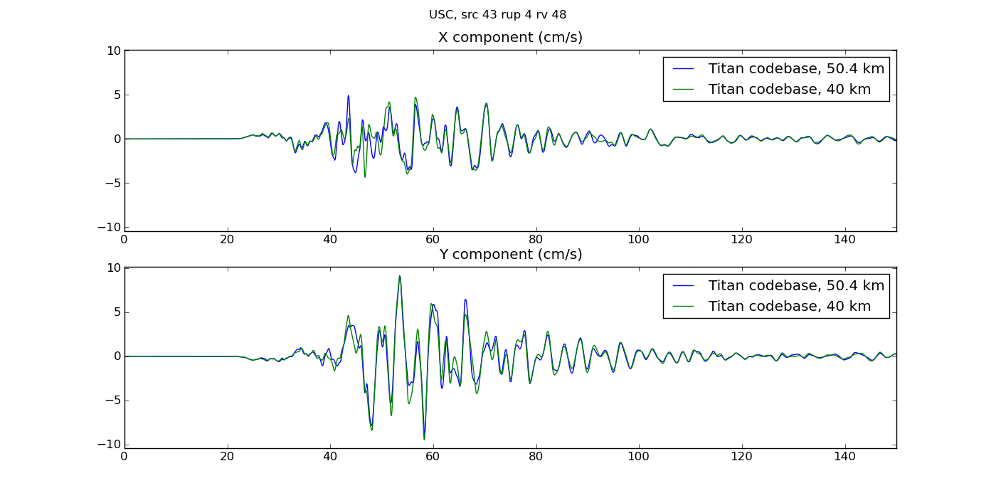
We accidentally ran with a depth of 50.4 km first. Here are seismogram plots illustrating the difference between running SGTs with depth of 40 km vs 50.4 km.
Velocity Model Verification
Cross-section plots of the velocity models are available here.
200 km cutoff effects
We are investigating the impact of the 200 km cutoff as it pertains to including/excluding northern SAF events. This is documented here: CCA N SAF Tests.
Impulse difference
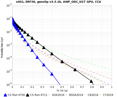
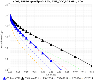
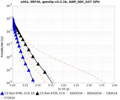
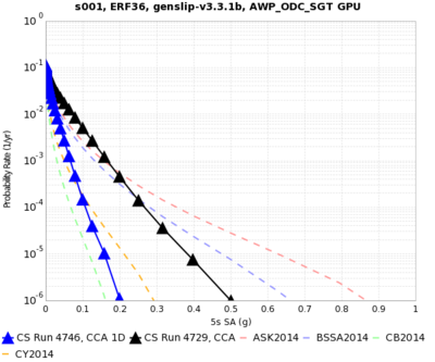
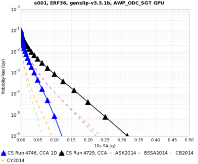
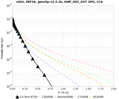
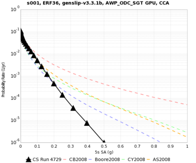
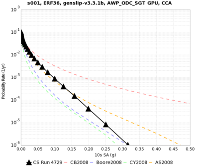
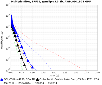
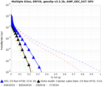
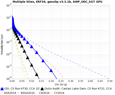
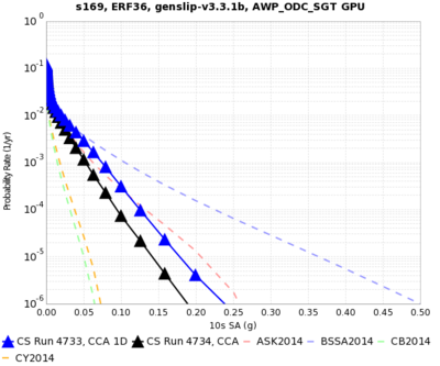
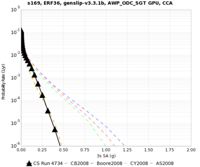
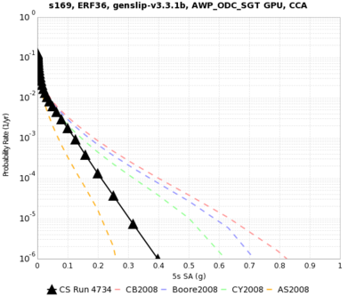
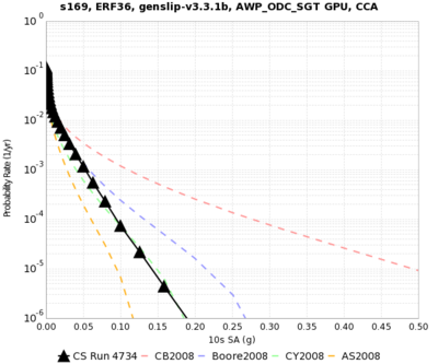
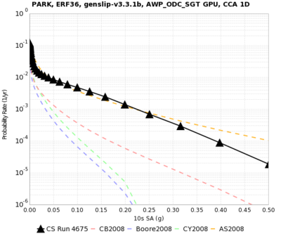
Here's a curve comparison showing the impact of fixing the impulse for s001 at 3, 5, and 10 sec.
Curve Results
| site | velocity model | 3 sec SA | 5 sec SA | 10 sec SA |
|---|---|---|---|---|
| s001 | 1D | |||
| 3D | ||||
| OSI | 1D | |||
| 3D | ||||
| s169 | 1D | |||
| 3D |
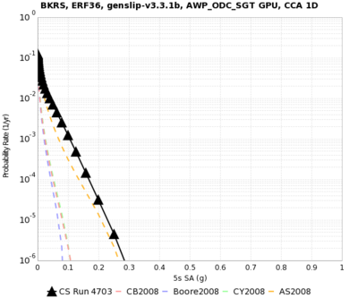
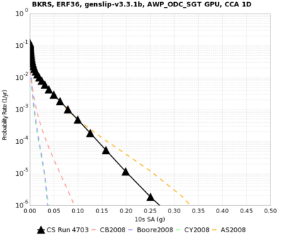
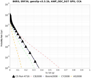
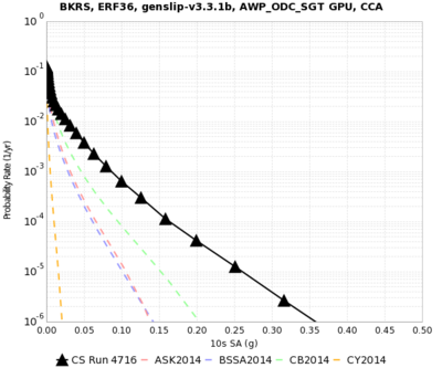
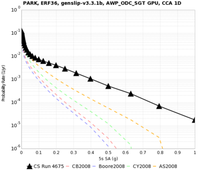
These results were calculated with the incorrect impulse.
| site | velocity model | 3 sec SA | 5 sec SA | 10 sec SA |
|---|---|---|---|---|
| BKRS | 1D | 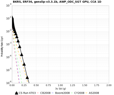
|
|
|
| 3D | 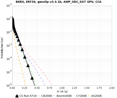
|
|
| |
| SBR | 1D | |||
| 3D | ||||
| PARK | 1D | 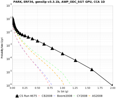
|
|
|
| 3D | 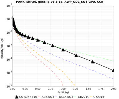
|
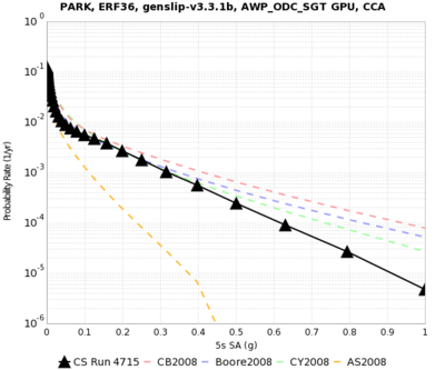
|
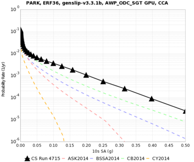
|
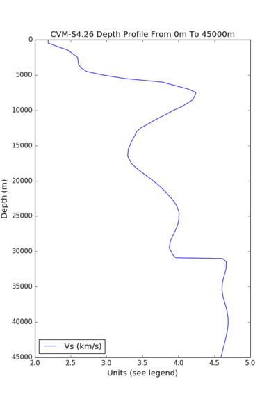
Velocity Profiles
| site | CCA profile (min Vs=900 m/s) | CVM-S4.26 profile (min Vs=500 m/s) |
|---|---|---|
| s001 | 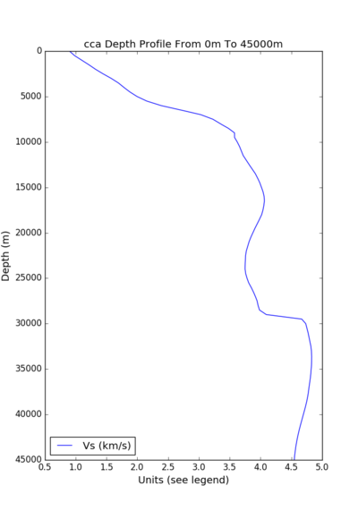
|
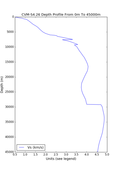
|
| OSI | 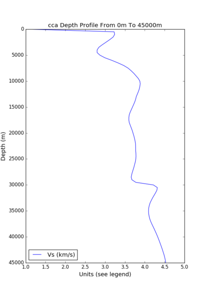
|
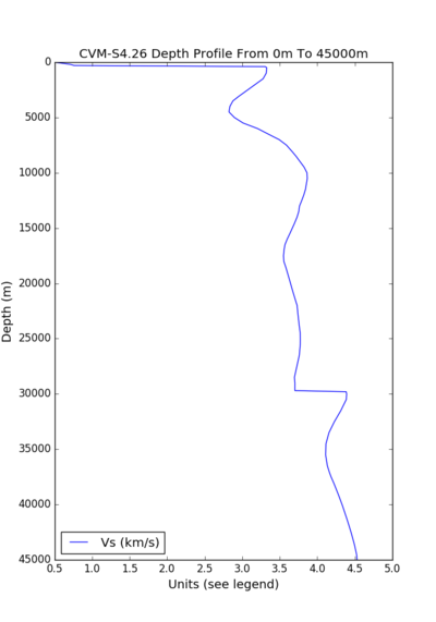
|
| s169 | 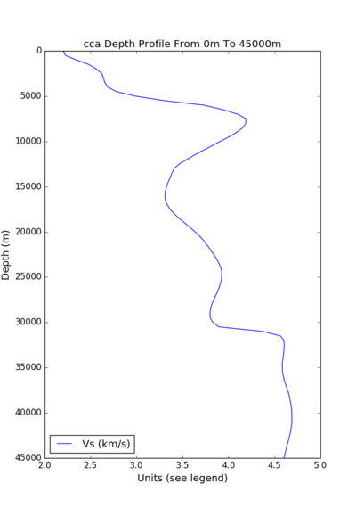
|
|
Seismogram plots
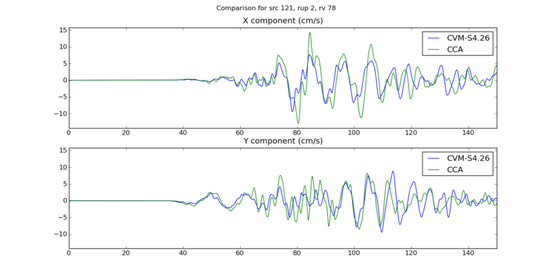
Below are plots comparing results from Study 15.4 to test results, which differ in velocity model, Vs min cutoff, dt, and grid spacing. We've selected two events: source 43, rupture 4, rupture variation 48, a M7.05 southern SAF event, and source 121, rupture 2, rupture variation 78, and M7.65 San Jacinto event.
| site | San Andreas event | San Jacinto event |
|---|---|---|
| s001 | 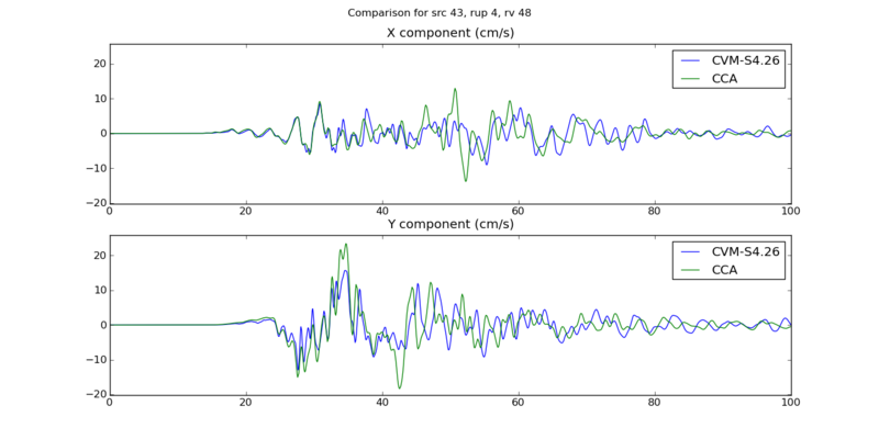
|
|
| OSI | 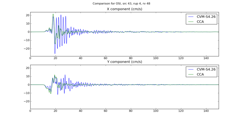
|
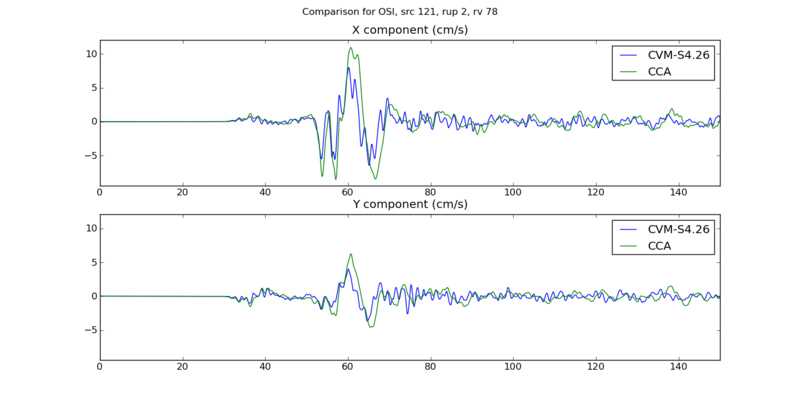
|
| s169 | 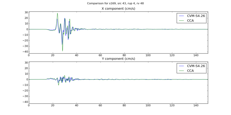
|
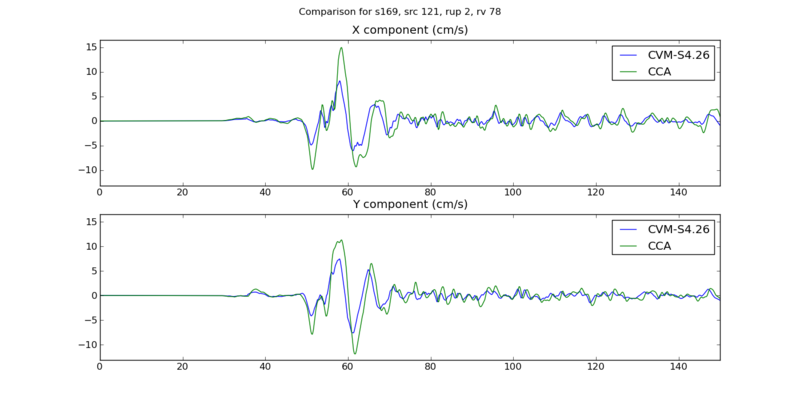
|
Rupture Variation Generator v5.2.3 (Graves & Pitarka 2015)
Plots related to verifying the rupture variation generator used in this study are available here: Rupture Variation Generator v5.2.3 Verification
Performance Enhancements (over Study 15.4)
Responses to Study 15.4 Lessons Learned
* Some of the DirectSynth jobs couldn't fit their SGTs into the number of SGT handlers, nor finish in the wallclock time. In the future, test against a larger range of volumes and sites.
We aren't quite sure which site will produce the largest volume, so we will take the largest volume produced among the test sites and add 10% when choosing DirectSynth job sizes.
* Some of the cleanup jobs aren't fully cleaning up.
We have had difficulty reproducing this in a non-production environment. We will add a cron job to send a daily email with quota usage, so we'll know if we're nearing quota.
* On Titan, when a pilot job doesn't complete successfully, the dependent pilot jobs remain in a held state. This isn't reflected in qstat, so a quick look doesn't show that some of these jobs are being held and will never run. Additionally, I suspect that pilot jobs exit with a non-zero exit code when there's a pile-up of workflow jobs, and some try to sneak in after the first set of workflow jobs runs on the pilot jobs, meaning that the job gets kicked out for exceeding wallclock time. We should address this next time.
We're not going to use pilot jobs this time, so it won't be an issue.
* On Titan, a few of the PostSGT and MD5 jobs didn't finish in the 2 hours, so they had to be run on Rhea by hand, which has a longer permitted wallclock time. We should think about moving these kind of processing jobs to Rhea in the future.
The SGTs for Study 16.9 will be smaller, so these jobs should finish faster. PostSGT has two components, reformatting the SGTs and generating the headers. By increasing from 2 nodes to 4, we can decrease the SGT reformatting time to about 15 minutes, and the header generation also takes about 15 minutes. We investigated setting up the workflow to run the PostSGT and MD5 jobs only on Rhea, but had difficulty getting the rvgahp server working there. Reducing the runtime of the SGT reformatting and separating out the MD5 sum should fix this issue for this study.
* When we went back to do to CyberShake Study 15.12, we discovered that it was common for a small number of seismogram files in many of the runs to have an issue wherein some rupture variation records were repeated. We should more carefully check the code in DirectSynth responsible for writing and confirming correctness of output files, and possibly add a way to delete and recreate RVs with issues.
We've fixed the bug that caused this in DirectSynth. We have changed the insertion code to abort if duplicates are detected.
Workflows
- We will run CyberShake workflows end-to-end on Titan, using the RVGAHP approach with Condor rather than pilot jobs.
- We will bypass the MD5sum check at the start of post-processing if the SGT and post-processing are being run back-to-back on the same machine.
Database
- We have migrated data from past studies off the production database, which will hopefully improve database performance from Study 15.12.
Lessons Learned
- Include plots of velocity models as part of readiness review when moving to new regions.
- Formalize process of creating impulse. Consider creating it as part of the workflow based on nt and dt.
Codes
Output Data Products
Below is a table of planned output products, both what we plan to compute and what we plan to put in the database.
| Type of product | Periods/subtypes computed and saved in files | Periods/subtypes inserted in database |
|---|---|---|
| PSA | 88 values X and Y components at 44 periods: 10, 9.5, 9, 8.5, 8, 7.5, 7, 6.5, 6, 5.5, 5, 4.8, 4.6, 4.4, 4.2, 4, 3.8, 3.6, 3.4, 3.2, 2, 2.8, 2.6, 2.4, 2.2, 2, 1.66667, 1.42857, 1.25, 1.11111, 1, .66667, .5, .4, .33333, .285714, .25, .22222, .2, .16667, .142857, .125, .11111, .1 sec |
4 values Geometric mean for 4 periods: 10, 5, 3, 2 sec |
| RotD | 44 values RotD100, RotD50, and RotD50 angle for 22 periods: 1.0, 1.2, 1.4, 1.5, 1.6, 1.8, 2.0, 2.2, 2.4, 2.6, 2.8, 3.0, 3.5, 4.0, 4.4, 5.0, 5.5, 6.0, 6.5, 7.5, 8.5, 10.0 sec |
14 values RotD100, RotD50, and RotD50 angle for 7 periods: 10, 7.5, 5, 4, 3, 2, 1.5 sec |
| Durations | 18 values For X and Y components, energy integral, Arias intensity, cumulative absolute velocity (CAV), and for both velocity and acceleration, 5-75%, 5-95%, and 20-80%. |
None |
| Hazard Curves | N/A | 18 curves Geometric mean: 10, 5, 3, 2 sec RotD100: 10, 7.5, 5, 4, 3, 2, 1.5 sec RotD100: 10, 7.5, 5, 4, 3, 2, 1.5 sec |
Computational and Data Estimates
Computational Time
Since we are using a min Vs=900 m/s, we will use a grid spacing of 175 m, and dt=0.00875, nt=23000 in the SGT simulation (and 0.0875 in the seismogram synthesis).
For computing these estimates, we are using a volume of 420 km x 1160 km x 50 km, or 2400 x 6630 x 286 grid points. This is about 4.5 billion grid points, approximately half the size of the Study 15.4 typical volume. We will run the SGTs on 160-200 GPUs.
We estimate that we will run 75% of the sites from each model on Blue Waters, and 25% on Titan. This is because we are charged less for Blue Waters sites (we are charged for the Titan GPUs even if we don't use them), and we have more time available on Blue Waters. However, we will use a dynamic approach during runtime, so the resulting numbers may differ.
Study 15.4 SGTs took 740 node-hours per component. From this, we assume:
750 node-hours x (4.5 billion grid points in 16.9 / 10 billion grid points in 15.4) x ( 23k timesteps in 16.9 / 40k timesteps in 15.4 ) ~ 200 node-hours per component for Study 16.9.
Study 15.4 post-processing took 40k core-hrs. From this, we assume:
40k core-hrs x ( 2.3k timesteps in 16.9 / 4k timesteps in 15.4 ) = 23k core-hrs = 720 node-hrs on Blue Waters, 1440 node-hrs on Titan.
Titan
Pre-processing (CPU): 100 node-hrs/site x 219 sites = 21,900 node-hours.
SGTs (GPU): 400 node-hrs per site x 219 sites = 87,600 node-hours.
Post-processing (CPU): 1440 node-hrs per site x 213 sites = 315,360 node-hours.
Total: 15.9M SUs ((21,900 + 87,600 + 315,360) x 30 SUs/node-hr + 25% margin)
We have 23M SUs available on Titan.
Blue Waters
Pre-processing (CPU): 100 node-hrs/site x 657 sites = 65,700 node-hours.
SGTs (GPU): 400 node-hrs per site x 657 sites = 262,800 node-hours.
Post-processing (CPU): 720 node-hrs per site x 657 sites = 473,000 node-hours.
Total: 1.00M node-hrs ((65,700 + 262,800 + 473,000) + 25% margin)
We have 3.04M node-hrs available on Blue Waters.
Storage Requirements
We plan to calculate geometric mean, RotD values, and duration metrics for all seismograms. We will use Pegasus's cleanup capabilities to avoid exceeding quotas.
Titan
Purged space to store intermediate data products: (900 GB SGTs + 60 GB mesh + 900 GB reformatted SGTs)/site x 219 sites = 398 TB
Purged space to store output data: (15 GB seismograms + 0.2 GB PSA + 0.2 GB RotD + 0.2 GB duration) x 219 sites = 3.3 TB
Blue Waters
Purged space to store intermediate data products: (900 GB SGTs + 60 GB mesh + 900 GB reformatted SGTs)/site x 657 sites = 1193 TB
Purged space to store output data: (15 GB seismograms + 0.2 GB PSA + 0.2 GB RotD + 0.2 GB duration) x 657 sites = 10.0 TB
SCEC
Archival disk usage: 13.3 TB seismograms + 0.1 TB PSA files + 0.1 TB RotD files + 0.1 TB duration files on scec-02 (has 109 TB free) & 24 GB curves, disaggregations, reports, etc. on scec-00 (109 TB free)
Database usage: (4 rows PSA [@ 2, 3, 5, 10 sec] + 12 rows RotD [RotD100 and RotD50 @ 2, 3, 4, 5, 7.5, 10 sec] + 8 rows duration [X and Y comps, acceleration and velocity, 5-75% and 5-95%])/rupture variation x 500K rupture variations/site x 876 sites = 10.5 billion rows x 125 bytes/row = 1.2 TB (3.9 TB free on moment.usc.edu disk)
Temporary disk usage: 1 TB workflow logs. scec-02 has 109 TB free.
Production Checklist
Check CISN stations; preference for broadband and PG&E stationsAdd DBCN to station list.- Complete the database migration outlined in 2016_CyberShake_database_migration.
Install 1D model in UCVM 15.10.0 on Blue Waters and Titan.Decide on 3D velocity model to use.Upgrade Condor on shock to v8.4.8.- Get the Pegasus Dashboard up and running.
Generate test hazard curves for 1D and 3D velocity models for 3 overlapping box sites- Run the same site on both Blue Waters and Titan.
Generate test hazard curves for 1D and 3D velocity models for 3 central CA sites.Calculate hazard curves for sites which include northern SAF events inside 200 km cutoff, with and without those events.- Confirm test results with science group.
Determine CyberShake volume for corner points in Central CA region, and if we need to modify the 200 km cutoff.Modify submit job on shock to distribute end-to-end workflows between Blue Waters and Titan.Add new velocity models into CyberShake database.Create XML file describing study for web monitoring toolAdd new sites to database.Determine size and length of jobs.Create Blue Waters and Titan daily cronjobs to monitor quota.Check scalability of reformat-awp-mpi code.Test rvgahp server on Rhea for PostSGT and MD5 jobs.Edit submission script to disable MD5 checks if we are submitting an integrated workflow to 1 system.Upgrade Pegasus on shock to 4.6.2.Add duration calculation to DirectSynth.- Verify DirectSynth duration calculation.
Reduce DirectSynth output.Generate hazard maps for region using GMPEs with and without 200 km cutoff.- Tag code in repository.
- Add check to abort SGTs if BLOCK_SIZE_Z is set incorrectly.
Integrate version of rupture variation generator in the BBP into CyberShake.Add new rupture variation generator to DB.Populate DB with new rupture variations.Check that monitord is being populated to sqlite databases.Change curve calc script to use NGA-2s.Add database argument to all OpenSHA jobs.Test running rvgahp daemon on dtn nodes.Verify with Rob that we should be using multi-segment version of rupture variation generator.Look at applying concurrency limits to transfer jobs.Ask HPC staff if we should use hpc-transfer instead of hpc-scec.Switch workflow to using hpc-transfer.- Scalability test of rvgahp on Titan
