CyberShake Study 22.12
CyberShake Study 22.10 is a proposed study in Southern California which will include deterministic low-frequency (0-1 Hz) and stochastic high-frequency (1-50 Hz) simulations. We will use the Graves & Pitarka (2022) rupture generator and the high frequency modules from the SCEC Broadband Platform v22.4.
Contents
- 1 Status
- 2 Data Products
- 3 Science Goals
- 4 Technical Goals
- 5 Sites
- 6 Velocity Model
- 7 Rupture Generator
- 8 High-frequency codes
- 9 Spectral Content around 1 Hz
- 10 Seismogram Length
- 11 Verification
- 12 Updates and Enhancements
- 13 Output Data Products
- 14 Computational and Data Estimates
- 15 Lessons Learned
- 16 Stress Test
- 17 Performance Metrics
- 18 Production Checklist
- 19 Presentations, Posters, and Papers
Status
This study is in the planning phase. We estimate calculations will begin in October 2022.
Data Products
Data products will be posted here when the study is completed.
Science Goals
The science goals for this study are:
- Calculate a regional CyberShake model for southern California using an updated rupture generator.
- Calculate an updated broadband CyberShake model.
- Sample variability in rupture velocity as part of the rupture generator.
Technical Goals
The technical goals for this study are:
- Use an optimized OpenMP version of the post-processing code.
- Bundle the SGT and post-processing jobs to run on large Condor glide-ins, taking advantage of queue policies favoring large jobs.
Sites
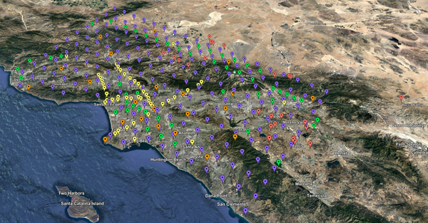
We will use the standard 335 southern California sites (same as Study 21.12). The order of execution will be:
- Sites of interest
- 20 km grid
- 10 km grid
- Selected 5 km grid sites
Velocity Model
We are planning to use CVM-S4.26 with a GTL applied, and the CVM-S4 1D background model outside of the region boundaries.
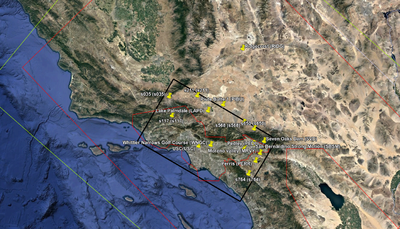
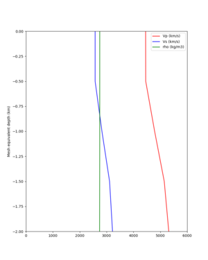
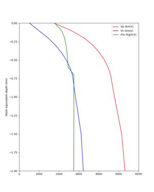
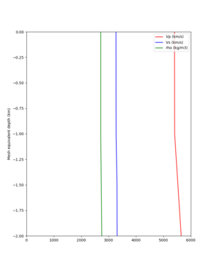
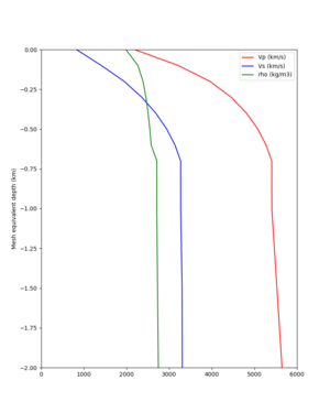
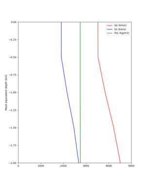
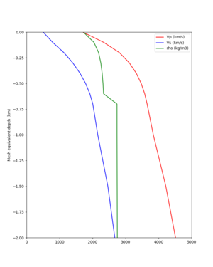
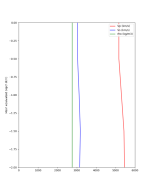
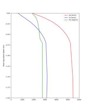
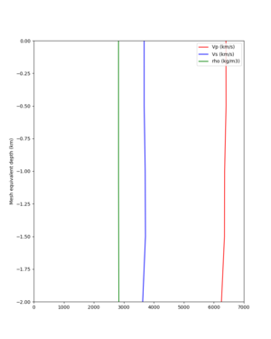
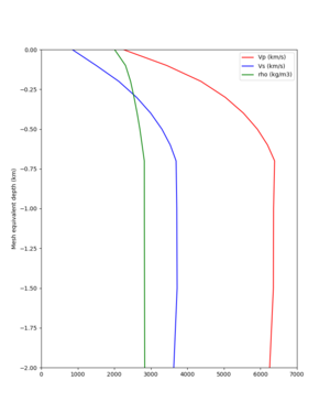
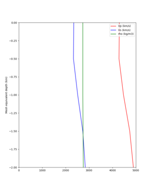
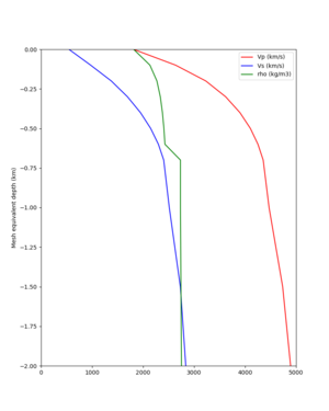
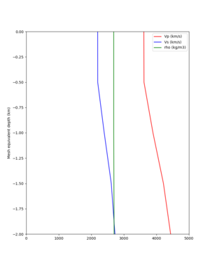
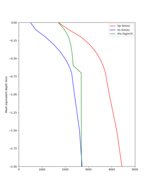
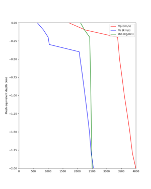
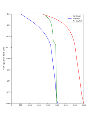
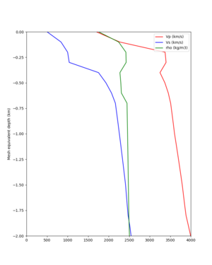
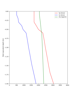
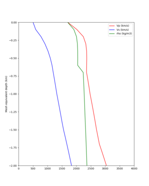
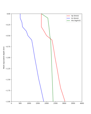
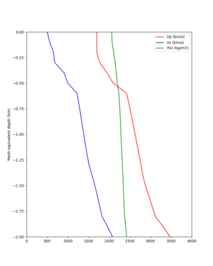
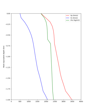
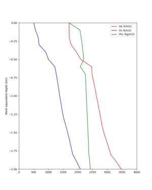
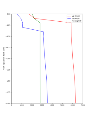
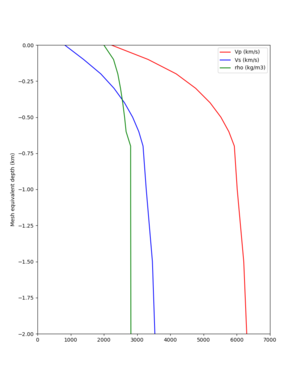
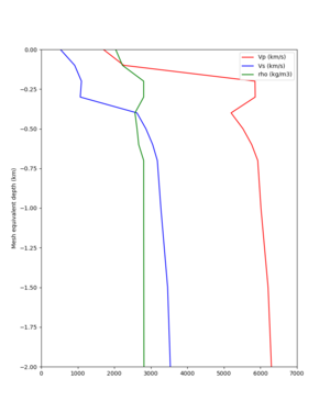
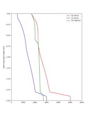
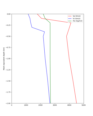
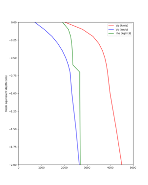
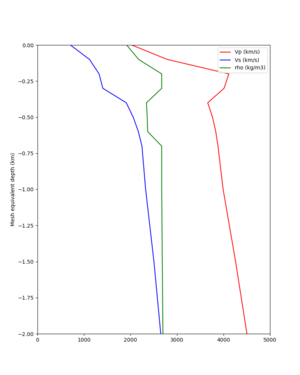
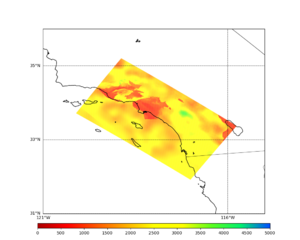
We are investigating applying the Ely-Jordan GTL down to 700 m instead of the default of 350m. We extracted profiles for a series of southern California CyberShake sites, with no GTL, a GTL applied down to 350m, and a GTL applied down to 700m.
Sites (the CVM-S4.26 basins are outlined in red):
These are for sites outside of the CVM-S4.26 basins:
| Site | No GTL | 700m GTL | Smaller value, extracted from mesh |
|---|---|---|---|
| LAPD | |||
| s764 | |||
| s568 | |||
| s035 | |||
| PERR | |||
| MRVY | |||
| s211 |
These are for sites inside of the CVM-S4.26 basins:
| Site | No GTL | 700m GTL | Smaller value |
|---|---|---|---|
| s117 | |||
| USC | |||
| WNGC | |||
| PEDL | |||
| SBSM | |||
| SVD |
Proposed Algorithm
Our proposed algorithm for generating the velocity model is as follows:
- Set the surface mesh point to a depth of 25m.
- Query the CVM-S4.26.M01 model ('cvmsi' string in UCVM) for each grid point.
- Calculate the Ely taper at that point using 700m as the transition depth.
- Compare the values before and after the taper modification; at each grid point down to the transition depth, use the value from the method with the lower Vs value.
- Check values for Vp/Vs ratio, minimum Vs, Inf/NaNs, etc.
Value constraints
We impose the following constraints on velocity mesh values:
- Vp >= 1700 m/s. If lower, Vp is set to 1700.
- Vs >= 500 m/s. If lower, Vs is set to 500.
- rho >= 1700 km/m3. If lower, rho is set to 1700.
- Vp/Vs >= 1.45. If not, Vs is set to Vp/1.45.
We will add the following additional constraints:
- If Vs<500 m/s, calculate the Vp/Vs ratio, set Vs=500, then set Vp=Vs*(Vp/Vs ratio).
- Apply Vp clamp after Vs check.
Cross-sections
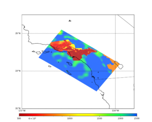
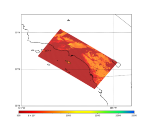
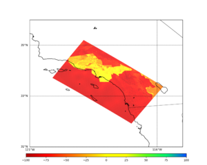
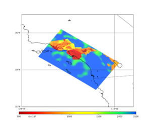
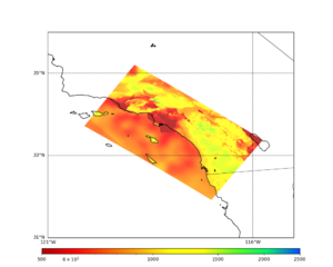
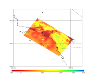
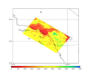
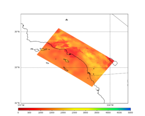
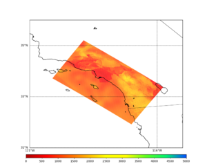
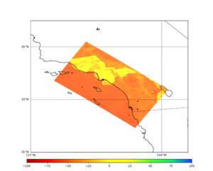
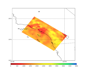
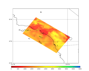
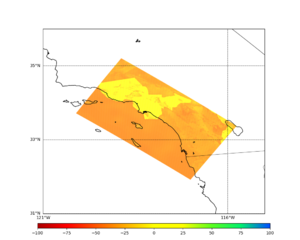
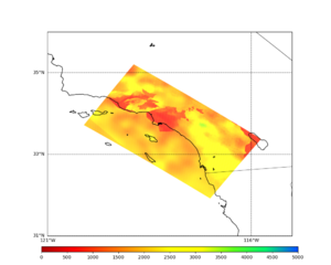
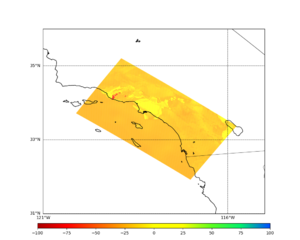
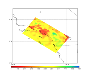
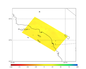
Below are cross-sections of the TEST site velocity model at depths down to 600m for CVM-S4.26.M01, the taper to 700m, the lesser of the two values, and the % difference.
Note that the top two slices use a different color scale.
| Depth | CVM-S4.26.M01 | Ely taper to 700m | Selecting smaller value | % difference, smaller value vs S4.26.M01 |
|---|---|---|---|---|
| 0m (queried at 25m depth) | ||||
| 100m | ||||
| 200m | ||||
| 300m | ||||
| 400m | ||||
| 500m | ||||
| 600m |
Implementation details
To support the Ely taper approach where the smaller value is selected, the following algorithmic changes were made to the CyberShake mesh generation code. Since the UCVM C API doesn't support removing models, we couldn't just add the 'elygtl' model - it would then be included in every query, and we need to run queries with and without it to make the comparison. We also must include the Ely interpolator, since all that querying the elygtl model does is populates the gtl part of the properties with the Vs30 value, and it's the interpolator which takes this and the crustal model info and generates the taper.
- The decomposition is done by either X-parallel or Y-parallel stripes, which have a constant depth. Check the depth to see if it is shallower than the transition depth.
- If so, initialize the elygtl model using ucvm_elygtl_model_init(), if uninitialized. Set the id to UCVM_MAX_MODELS-1. There's no way to get model id info from UCVM, so we use UCVM_MAX_MODELS-1 as it is 29, we are very unlikely to load 29 models, and therefore unlikely to have an id conflict.
- Change the depth value of the points to query to the transition depth. This is because we need to know the crustal model Vs value at the transition depth, so that the Ely interpolator can match it.
- Query the crustal model again, with the modified depths.
- Modify the 'domain' parameter in the properties data structure to UCVM_DOMAIN_INTERP, to indicate that we will be using an interpolator.
- Change the depth value of the points to query back to the correct depth, so that the interpolator can work correctly on them.
- Query the elygtl using ucvm_elygtl_model_query() and the correct depth.
- Call the interpolator for each point independently, using the correct depth.
- For each point, choose to use either the original crustal data or the Ely taper data, depending on which has the lower Vs.
In the future we plan for this approach to be implemented in UCVM, and we can simplify the CyberShake query code.
Impact on hazard
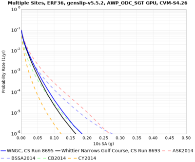
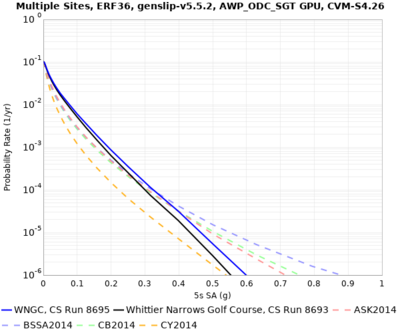
Below are hazard curves calculated with the old approach, and with the implementation described above.
Rupture Generator
Initial Findings
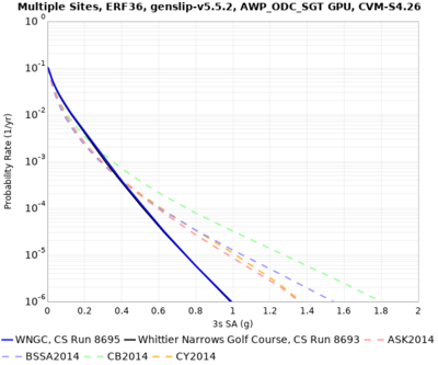
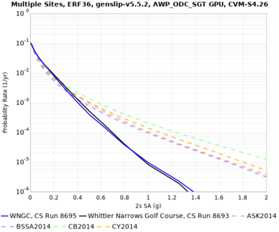
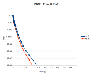
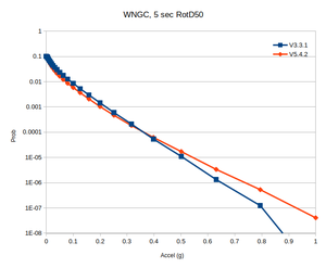
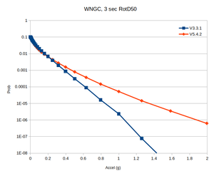
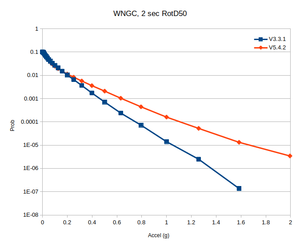
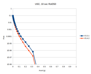
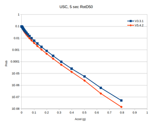
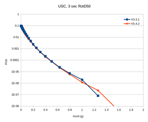
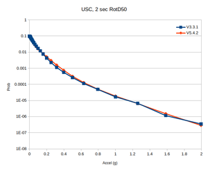
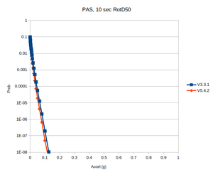
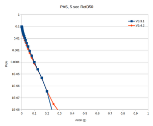
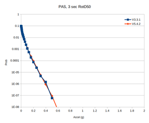
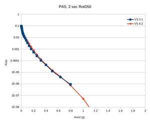
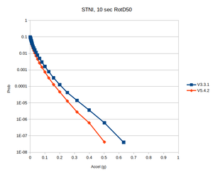
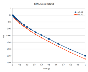
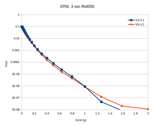
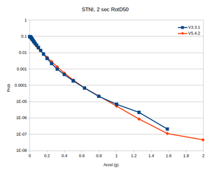
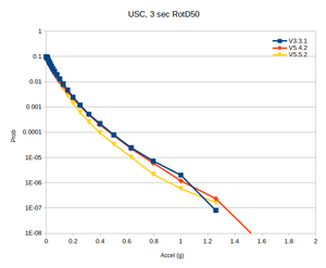
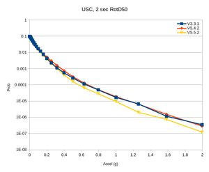
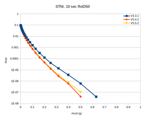
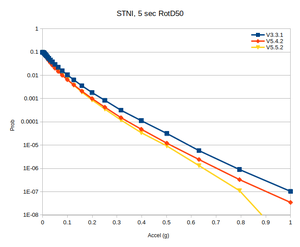
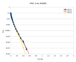
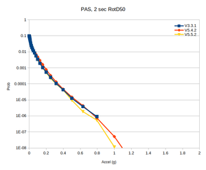
In determining what rupture generator to use for this study, we performed tests with WNGC, USC, PAS, and STNI, and compared hazard curves generated with v5.4.2 to those from Study 15.4:
| Site | 10 sec | 5 sec | 3 sec | 2 sec |
|---|---|---|---|---|
| WNGC | ||||
| USC | ||||
| PAS | ||||
| STNI |
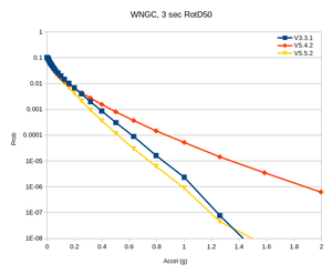
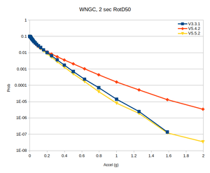
Digging in further, it appears the elevated hazard curves for WNGC at 2 and 3 seconds are predominately due to large-magnitude southern San Andreas events producing larger ground motions.
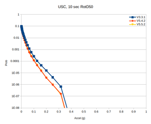
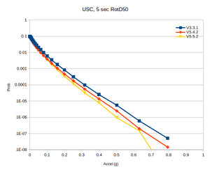
USC, PAS, and STNI also all see larger ground motions at 2-3 seconds from these same events, but the effect isn't as strong, so it only shows up in the tails of the hazard curves.
We honed in on source 68, rupture 7, a M8.45 on the southern San Andreas which produced the largest WNGC ground motions at 3 seconds, up to 5.1g. We calculated spectral plots for v3.3.1 and v5.4.2 for all 4 sites:
| Site | v3.3.1 | v5.4.2 |
|---|---|---|
| WNGC | ||
| USC | ||
| PAS | ||
| STNI |
v5.5.2
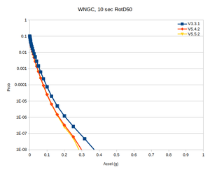
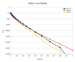
We decided to try v5.5.2 of the rupture generator, which typically has less spectral content at short periods:
| Site | v3.3.1 | v5.4.2 | v5.5.2 |
|---|---|---|---|
| WNGC |
Hazard Curves
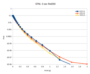
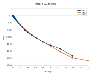
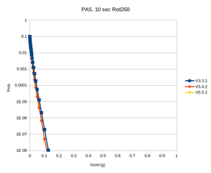
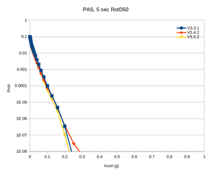
Comparison hazard curves for the three rupture generators, using no taper
| Site | 10 sec | 5 sec | 3 sec | 2 sec |
|---|---|---|---|---|
| WNGC | ||||
| USC |
Comparison curves for the three rupture generators, using the smaller value in the velocity model.
| Site | 10 sec | 5 sec | 3 sec | 2 sec |
|---|---|---|---|---|
| STNI | ||||
| PAS |
Scatter Plots
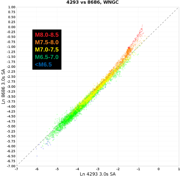
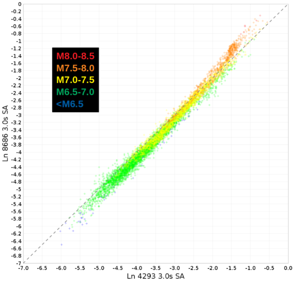
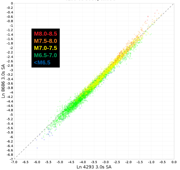
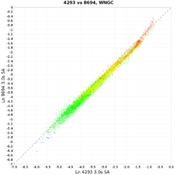
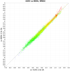
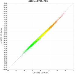
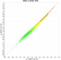
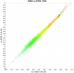
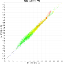
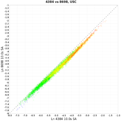
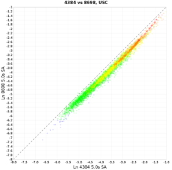
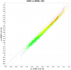
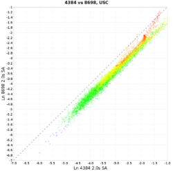
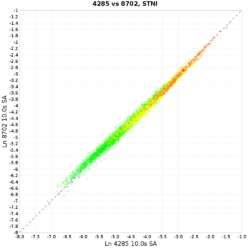
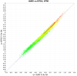
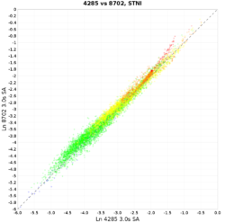
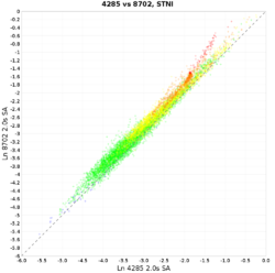
Scatter plots, comparing results with v5.5.2 to results from Study 15.12 by plotting the mean ground motion for each rupture. The colors are magnitude bins (blue: <M6.5; green: M6.5-7; yellow: M7-7.5; orange: M7.5-8; red: M8+).
| Site | 10 sec | 5 sec | 3 sec | 2 sec |
|---|---|---|---|---|
| WNGC | ||||
| PAS | ||||
| USC | ||||
| STNI |
High-frequency codes
For this study, we will use the Graves & Pitarka high frequency module (hb_high) from the Broadband Platform v22.4, hb_high_v6.0.5. We will use the following parameters. Parameters in bold have been changed for this study.
| Parameter | Value |
|---|---|
| stress_average | 50 |
| rayset | 2,1,2 |
| siteamp | 1 |
| nbu | 4 (not used) |
| ifft | 0 (not used) |
| flol | 0.02 (not used) |
| fhil | 19.9 (not used) |
| irand | Seed used for generating SRF |
| tlen | Seismogram length, in sec |
| dt | 0.01 |
| fmax | 10 (not used) |
| kappa | 0.04 |
| qfexp | 0.6 |
| mean_rvfac | 0.775 |
| range_rvfac | 0.1 |
| rvfac | Calculated using BBP hfsims_cfg.py code |
| shal_rvfac | 0.6 |
| deep_rvfac | 0.6 |
| czero | 2 |
| c_alpha | -99 |
| sm | -1 |
| vr | -1 |
| vsmoho | 999.9 |
| nlskip | -99 |
| vpsig | 0 |
| vshsig | 0 |
| rhosig | 0 |
| qssig | 0 |
| icflag | 1 |
| velname | -1 |
| fa_sig1 | 0 |
| fa_sig2 | 0 |
| rvsig1 | 0.1 |
| ipdur_model | 11 |
| ispar_adjust | 1 |
| targ_mag | -1 |
| fault_area | -1 |
| default_c0 | 57 |
| default_c1 | 34 |
Spectral Content around 1 Hz
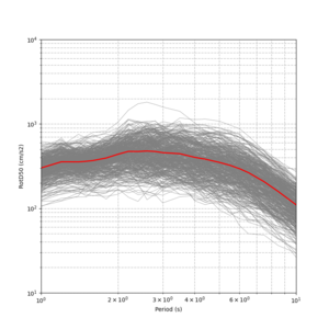
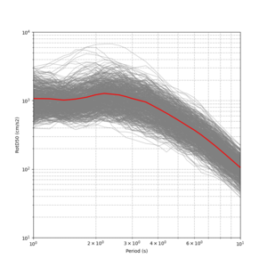
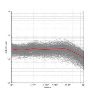
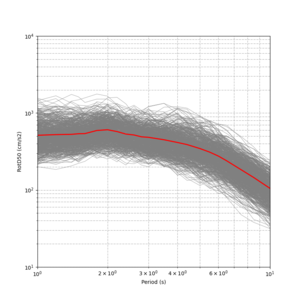
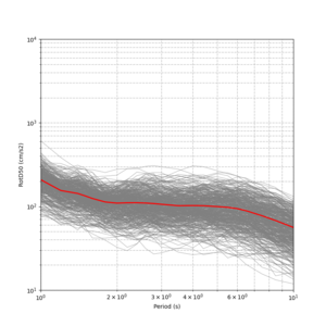
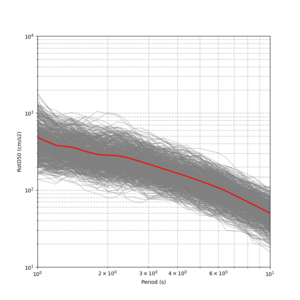
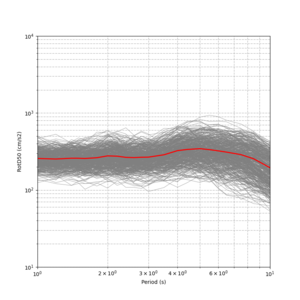
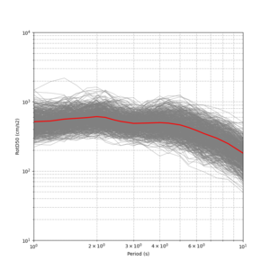
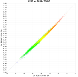
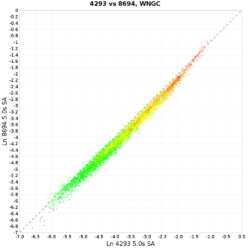
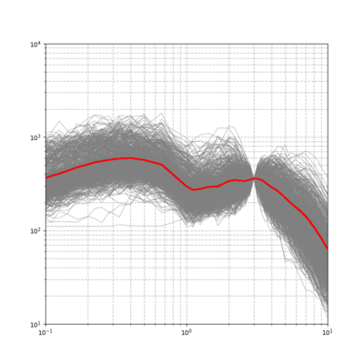
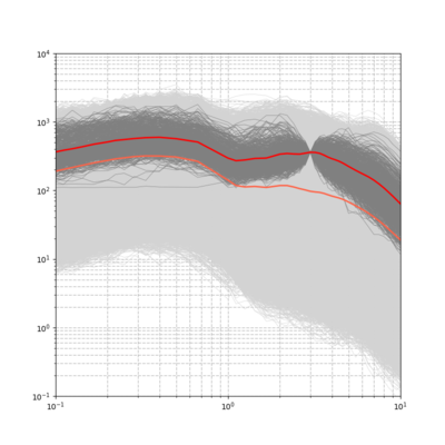
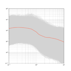
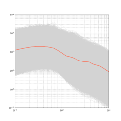
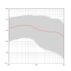
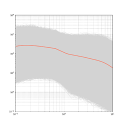
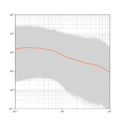
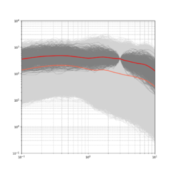
We investigated the spectral content of the Broadband CyberShake results in the 0.5-3 second range, to look for any discontinuities.
The plot below is from WNGC, Study 15.12 (run ID 4293).
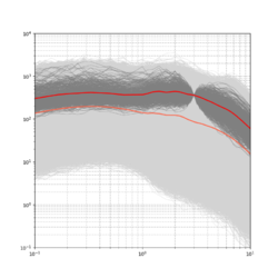
Below is a plot of the hypocenters from the 706 rupture variations which meet the target.
These events have a different distribution than the rupture variations as a whole.
| Fault | Percent of target RVs | Percent of all RVs |
|---|---|---|
| San Andreas | 60 | 44 |
| Elsinore | 21 | 9 |
| San Jacinto | 13 | 8 |
| Other | 6 | 39 |
Additionally, 88% of the selected events have a magnitude greater than the average for their source. 4% are average, and 8% are lower.
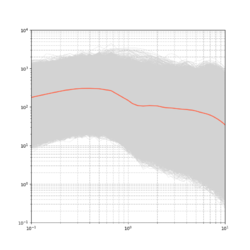
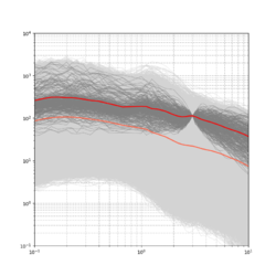
Below is a spectral plot but which includes all rupture variations and the overall mean (in orange).
Additional Sites
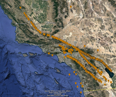
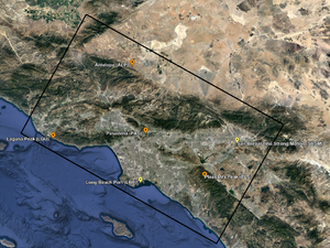
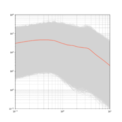
We created spectral plots for 7 additional sites (STNI, SBSM, PAS, LGU, LBP, ALP, PLS), located here:
| STNI | SBSM | PAS | LGU | LBP | ALP | PLS |
|---|---|---|---|---|---|---|
v5.5.2
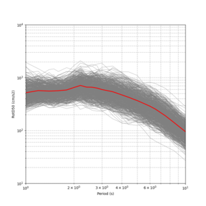
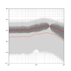
We created spectral plots using results produced with rupture generator v5.5.2. These results have a much less noticeable slope around 1 sec.
| WNGC | PAS | USC | STNI |
|---|---|---|---|
Seismogram Length
Originally we proposed a seismogram length of 500 sec. We examined seismograms for our most distance event-station pairs for this study and concluded that most stop having any meaningful signal by around 325 sec. Thus, we are reducing the seismogram length to 400 sec to ensure some margin of error.
Verification
Updates and Enhancements
Output Data Products
File-based data products
We plan to produce the following data products, which will be stored at CARC:
Deterministic
- Seismograms: 2-component seismograms, 10000 timesteps (500 sec) each.
- PSA: X and Y spectral acceleration at 44 periods (10, 9.5, 9, 8.5, 8, 7.5, 7, 6.5, 6, 5.5, 5, 4.8, 4.6, 4.4, 4.2, 4, 3.8, 3.6, 3.4, 3.2, 3, 2.8, 2.6, 2.4, 2.2, 2, 1.66667, 1.42857, 1.25, 1.11111, 1, .66667, .5, .4, .33333, .285714, .25, .22222, .2, .16667, .142857, .125, .11111, .1 sec)
- RotD: PGV, and RotD50, the RotD50 azimuth, and RotD100 at 25 periods (20, 15, 12, 10, 8.5, 7.5, 6.5, 6, 5.5, 5, 4.4, 4, 3.5, 3, 2.8, 2.6, 2.4, 2.2, 2, 1.7, 1.5, 1.3, 1.2, 1.1, 1)
- Durations: for X and Y components, energy integral, Arias intensity, cumulative absolute velocity (CAV), and for both velocity and acceleration, 5-75%, 5-95%, and 20-80%.
Broadband
- Seismograms: 2-component seismograms, 50000 timesteps (500 sec) each.
- PSA: X and Y spectral acceleration at 44 periods (10, 9.5, 9, 8.5, 8, 7.5, 7, 6.5, 6, 5.5, 5, 4.8, 4.6, 4.4, 4.2, 4, 3.8, 3.6, 3.4, 3.2, 3, 2.8, 2.6, 2.4, 2.2, 2, 1.66667, 1.42857, 1.25, 1.11111, 1, .66667, .5, .4, .33333, .285714, .25, .22222, .2, .16667, .142857, .125, .11111, .1 sec)
- RotD: PGA, PGV, and RotD50, the RotD50 azimuth, and RotD100 at 66 periods (20, 15, 12, 10, 8.5, 7.5, 6.5, 6, 5.5, 5, 4.4, 4, 3.5, 3, 2.8, 2.6, 2.4, 2.2, 2, 1.7, 1.5, 1.3, 1.2, 1.1, 1, 0.85, 0.75, 0.65, 0.6, 0.55, 0.5, 0.45, 0.4, 0.35, 0.3, 0.28, 0.26, 0.24, 0.22, 0.2, 0.17, 0.15, 0.13, 0.12, 0.11, 0.1, 0.085, 0.075, 0.065, 0.06, 0.055, 0.05, 0.045, 0.04, 0.035, 0.032, 0.029, 0.025, 0.022, 0.02, 0.017, 0.015, 0.013, 0.012, 0.011, 0.01)
- Durations: for X and Y components, energy integral, Arias intensity, cumulative absolute velocity (CAV), and for both velocity and acceleration, 5-75%, 5-95%, and 20-80%.
Database data products
We plan to store the following data products in the database on moment:
Deterministic
- RotD50 and RotD100 for 6 periods (10, 7.5, 5, 4, 3, 2)
- Duration: acceleration 5-75% and 5-95%, for both X and Y
Broadband
- RotD50 and RotD100 for PGA, PGV, and 19 periods (10, 7.5, 5, 4, 3, 2, 1, 0.75, 0.5, 0.4, 0.3, 0.2, 0.1, 0.075, 0.05, 0.04, 0.03, 0.02, 0.01)
- Duration: acceleration 5-75% and 5-95%, for both X and Y
Computational and Data Estimates
Computational Estimates
We based these estimates on scaling from the average of sites USC, STNI, PAS, and WNGC, which have within 1% of the average number of variations per site.
| UCVM runtime | UCVM nodes | SGT runtime (both components) | SGT nodes | Other SGT workflow jobs | Summit Total | |
|---|---|---|---|---|---|---|
| 4 site average | 436 sec | 50 | 3776 sec | 67 | 8700 node-sec | 78.8 node-hrs |
78.8 node-hrs x 335 sites + 10% overrun margin gives us an estimate of 29.0k node-hours for SGT calculation.
| DirectSynth runtime | DirectSynth nodes | Summit Total | |
|---|---|---|---|
| 4 site average | 31500 | 100 | 875 |
875 node-hours x 335 sites + 10% overrun margin gives an estimate of 322k node-hours for post-processing.
| PMC runtime | PMC nodes | Summit Total | |
|---|---|---|---|
| 4 site average | 31005 | 92 | 792 |
1078 node-hrs x 335 sites + 10% overrun margin gives an estimate of 292k node-hours for broadband calculations.
Data Estimates
Summit
These estimates assume a 400 sec seismogram.
| Velocity mesh | SGTs size | Temp data | Output data | |
|---|---|---|---|---|
| 4 site average (GB) | 177 | 1533 | 1533 | 225 |
| Total for 335 sites (TB) | 57.8 | 501.4 | 501.4 | 73.6 |
CARC
We estimate 92.1 TB in output data, which will be transferred back to CARC.
shock-carc
The study should use approximately ??? GB in workflow log space on /home/shock. This drive has approximately ??? TB free.
moment database
The PeakAmplitudes table uses approximately 99 bytes per entry.
99 bytes/entry * 34 entries/event (11 det + 25 stoch) * 622,636 events/site * 335 sites = 654 GB. The drive on moment with the mysql database has 771 GB free, so we will plan to migrate Study 17.3 and Study 18.8 off of moment to free up additional room.
Lessons Learned
Stress Test
Performance Metrics
Production Checklist
Science to-dos
Run WNGC and USC with updated velocity model.- Redo validation for Northridge and Landers with updated velocity model.
- For each validation event, calculate BBP results, CS results
- Check for spectral discontinuities around 1 Hz
Decide if we should stick with rvfrac=0.8 or allow it to varyDetermine appropriate SGT, low-frequency, and high-frequency seismogram durations- Update high-frequency Vs30 to use released Thompson values
Modify RupGen-v5.5.2 into CyberShake APITest RupGen-v5.5.2- Update to using v6.1.1 of hb_high.
Technical to-dos
Integrate refactoring of BBP codes into latest BBP releaseSwitch to using github repo version of CyberShake on SummitUpdate to latest UCVM (v22.7)Switch to optimized version of rupture generatorTest DirectSynth code with fixed memory leak from Frontera- Switch to using Pegasus-supported interface to Globus transfers
- Test bundled glide-in jobs for SGT and DirectSynth jobs
- Fix seg fault in PMC running broadband processing
Update curve generation to generate curves with more pointsTest OpenMP version of DirectSynthMigrate Study 18.8 from moment to focal.Delete Study 18.8 off of moment.- Optimize PeakAmplitudes table on moment.
Move Study 13.4 output files from CARC to OLCF HPSS.- Move Study 14.2 output files from CARC to OLCF HPSS.
- Switch to using OMP version of DS code by default.
- Review wiki content.
- Tag code.
