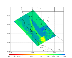
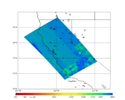
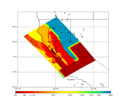
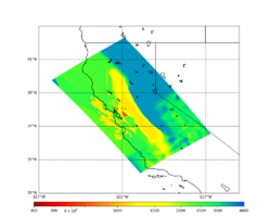
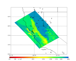
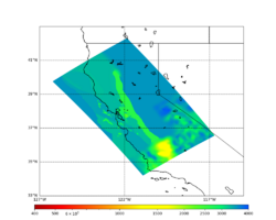
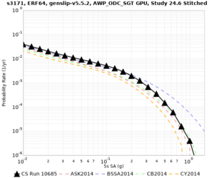
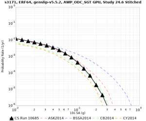
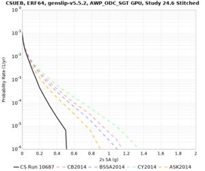
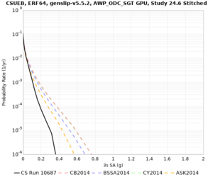
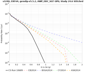
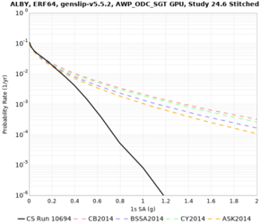
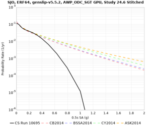
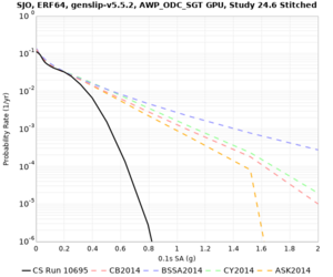
CyberShake Study 24.8
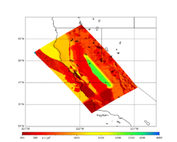
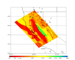
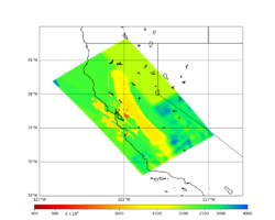
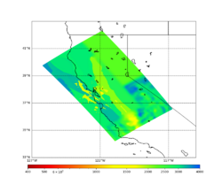
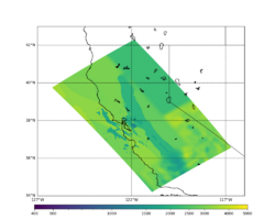
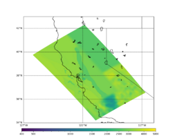
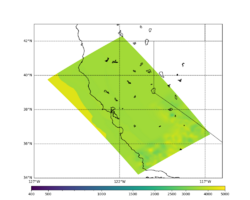
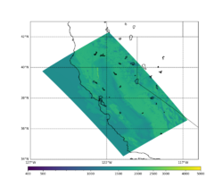
CyberShake Study 24.8 is a study in Northern California which includes deterministic low-frequency (0-1 Hz) and stochastic high-frequency (1-50 Hz) simulations. We will use the Graves & Pitarka (2022) rupture generator and the high frequency modules from the SCEC Broadband Platform v22.4. This study includes vertical component seismograms, period-dependent durations, and Fourier spectra IMs, and a reduction in minimum Vs to 400 m/s.
Contents
- 1 Status
- 2 Data Products
- 3 Science Goals
- 4 Technical Goals
- 5 Sites
- 6 Ruptures to Include
- 7 Velocity Model
- 7.1 Primary 3D model
- 7.2 Potential modification to gabbro regions
- 7.3 Background model
- 7.4 Cross-sections
- 7.4.1 Cross-sections, no smoothing, CVM-S4.26.M01 1D background
- 7.4.2 Cross-sections, smoothing, CVM-S4.26.M01 1D background
- 7.4.3 Cross-sections, no smoothing, Southern Sierra BBP 1D background
- 7.4.4 Cross-sections, no smoothing, extended SFCVM Sierra 1D background, CCA + taper
- 7.4.5 Cross-sections, smoothing, extended SFCVM Sierra 1D background, CCA + taper
- 7.4.6 Cross-sections, no smoothing, extended SFCVM Sierra 1D background with taper, CCA + taper
- 7.5 Candidate Model (RC1)
- 7.6 Vp/Vs Ratio Adjustment
- 7.7 Candidate Model (RC2)
- 7.8 Taper impact
- 8 Strain Green Tensors
- 9 Vertical Component
- 10 Rupture Generator
- 11 High-frequency codes
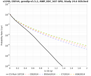
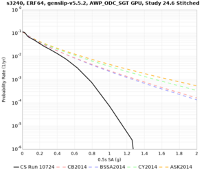
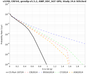
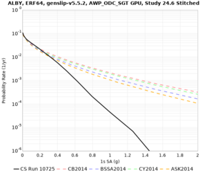
- 12 Hazard Curve Tests
- 13 Updates and Enhancements
- 14 Output Data Products
- 15 Computational and Data Estimates
- 16 Lessons Learned
- 17 Stress Test
- 18 Events During Study
- 19 Performance Metrics
- 20 Production Checklist
- 21 Presentations, Posters, and Papers
- 22 References
Status
This study was completed on 11/8/24 at 6:15:15 PST.
The low-frequency calculations finished on 10/30/24 at 04:52:52 PDT.
Study results are posted below.
Data Products
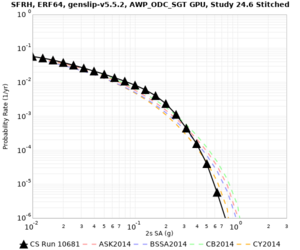
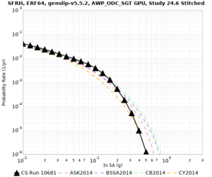
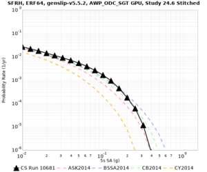
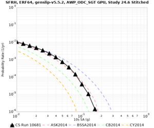
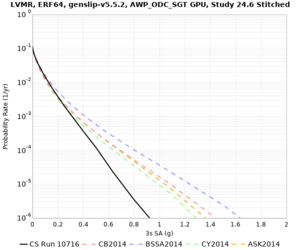
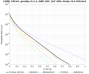
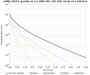
Low-frequency hazard maps are available here: Low-frequency Hazard Maps.
Low-frequency GMM comparisons are available here, using top velocity mesh value as Vs30 and Thompson Vs30.
Broadband hazard maps are available here: Broadband Hazard Maps.
Broadband GMM comparisons are available here: Broadband GMM Comparisons.
Science Goals
The science goals for this study are:
- To perform an updated broadband study for the greater Bay Area.
- To use an updated rupture generator and improved velocity model from Study 18.8.
- To use the same parameters as in Study 22.12 when possible to make comparisons between the studies simple.
Technical Goals
The technical goals for this study are:
- Use Frontier for the SGTs and Frontera for the post-processing and high-frequency calculations.
- Use a modified approach for the production database, to improve performance.
Sites
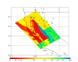
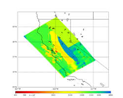
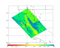
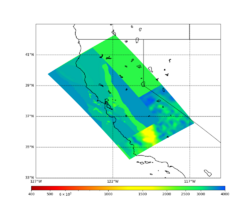
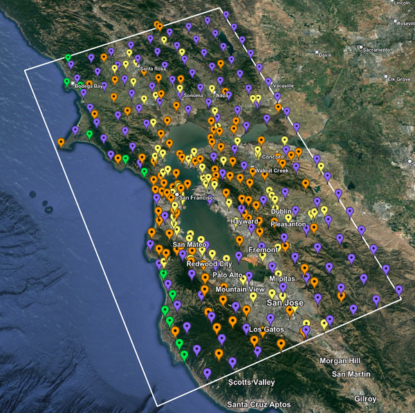
For this study, we chose to focus on a smaller region than in Study 18.8. Starting with the Study 18.8 region, we selected a smaller (180 km x 100 km) box extending roughly from San Jose to Santa Rosa, containing 315 sites.
|
Ruptures to Include
Summary: we decided to exclude the southern San Andreas events from Study 24.8. This was implemented by creating a new ERF with ID 64, which includes all the ERF 36 ruptures except for the southern San Andreas events.
Historically, we have determined which ruptures to include in a CyberShake run by calculating the distance between the site and the closest part of the rupture surface. If that distance is less than 200 km, we then include all ruptures which take place on that surface, including ruptures which may extend much farther away from the site than 200 km.
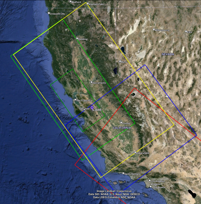
For Northern California sites, this means that sites around San Jose and south include southern San Andreas events (events which rupture the northernmost segment of the southern San Andreas) within 200 km. Since there are some UCERF2 ruptures which extend from the Parkfield segment all the way down to Bombay Beach, the simulation volumes for some of these Northern California sites cover most of the state. This was the case for Study 18.8 (sample volumes can be seen on this page). This required tiling together 3 3D models and a background 1D model.
To simplify the velocity model and reduce the volumes, we are investigating omitting southern San Andreas events from this study.
Source Contribution Curves
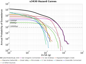
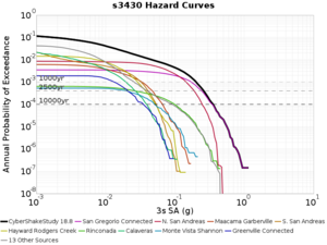
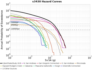
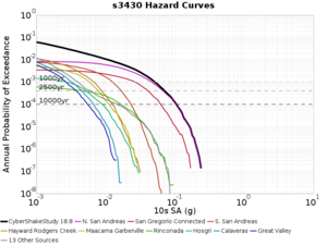
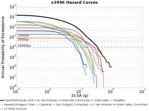
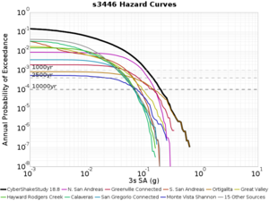
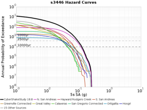
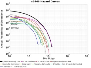
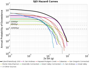
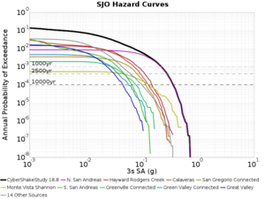
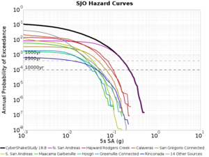
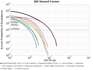
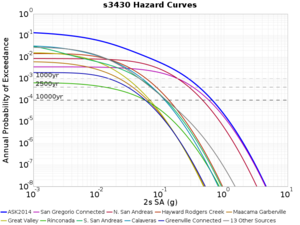
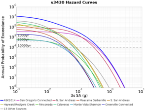
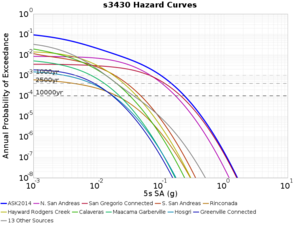
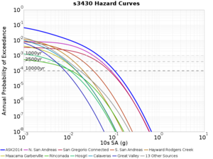
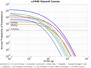
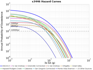
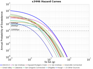
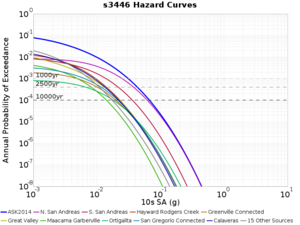
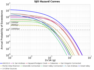
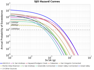
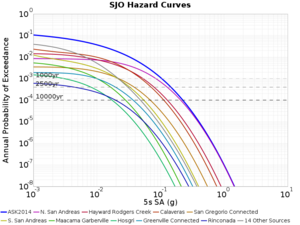
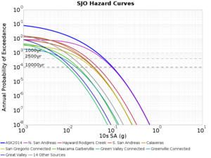
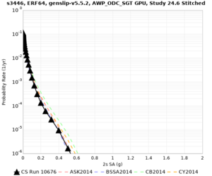
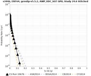
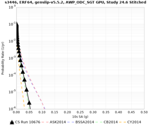
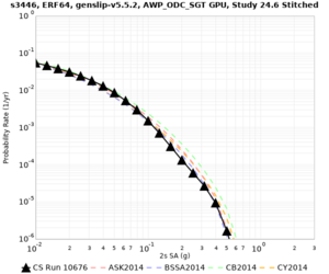
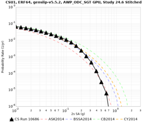
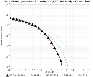
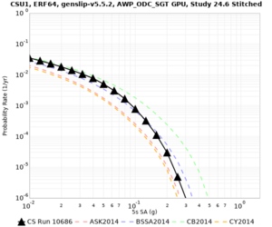
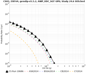
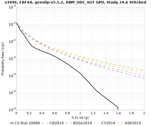
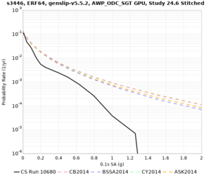
Below are source contribution curves for 3 sites: s3430 (southwest corner of the study region), s3446 (southeast corner of the study region), and SJO (San Jose). In general, the sSAF events are about the 3rd largest contributor at long periods and medium-to-long return periods.
| Site | 2 sec | 3 sec | 5 sec | 10 sec |
|---|---|---|---|---|
| s3430 | ||||
| s3446 | ||||
| SJO |
We also looked at the source contributions for these 3 sites from ASK 2014. In general, the sSAF events play a reduced role compared to the CyberShake results.
| Site | 2 sec | 3 sec | 5 sec | 10 sec |
|---|---|---|---|---|
| s3430 | ||||
| s3446 | ||||
| SJO |
Disaggregations
From Study 18.8, we looked at disaggregations for s3430, s3446, and SJO at 1e-3 (1000 yr), 4e-4 (2500 yr), and 1e-4 (10000 yr) probability levels, at 2 and 10 seconds. We list the top 3 contributing sources from the southern SAF, their magnitude ranges, and their contributing percentages.
The only significant contributions are for site s3446 at 10 second period. Those come from large events, with median magnitude 7.85 or higher.
s3430
| Period | 1e-3 | 4e-4 | 1e-4 |
|---|---|---|---|
| 2 sec | 80 (S. San Andreas;PK, M5.65-6.35), <0.01% 81 (S. San Andreas;PK+CH, M6.75-7.35), <0.01% 82 (S. San Andreas;PK+CH+CC, M7.15-7.65), <0.01% |
80 (S. San Andreas;PK, M5.65-6.35), <0.01% 81 (S. San Andreas;PK+CH, M6.75-7.35), <0.01% 82 (S. San Andreas;PK+CH+CC, M7.15-7.65), <0.01% |
80 (S. San Andreas;PK, M5.65-6.35), <0.01% 81 (S. San Andreas;PK+CH, M6.75-7.35), <0.01% 82 (S. San Andreas;PK+CH+CC, M7.15-7.65), <0.01% |
| 10 sec | 86 (S. San Andreas;PK+CH+CC+BB+NM+SM+NSB, M7.65-8.25), 0.01% 89 (S. San Andreas;PK+CH+CC+BB+NM+SM+NSB+SSB+BG+CO, M7.75-8.45), 0.01% 85 (S. San Andreas;PK+CH+CC+BB+NM+SM, M7.55-8.15), <0.01% |
89 (S. San Andreas;PK+CH+CC+BB+NM+SM+NSB+SSB+BG+CO, M7.75-8.45), <0.01% 80 (S. San Andreas;PK, M5.65-6.35), <0.01% 81 (S. San Andreas;PK+CH, M6.75-7.35), <0.01% |
80 (S. San Andreas;PK, M5.65-6.35), <0.01% 81 (S. San Andreas;PK+CH, M6.75-7.35), <0.01% 82 (S. San Andreas;PK+CH+CC, M7.15-7.65), <0.01% |
s3446
| Period | 1e-3 | 4e-4 | 1e-4 |
|---|---|---|---|
| 2 sec | 84 (S. San Andreas;PK+CH+CC+BB+NM, M7.45-7.95), <0.01% 89 (S. San Andreas;PK+CH+CC+BB+NM+SM+NSB+SSB+BG+CO, M7.75-8.45), <0.01% 80 (S. San Andreas;PK, M5.65-6.35), <0.01% |
80 (S. San Andreas;PK, M5.65-6.35), <0.01% 81 (S. San Andreas;PK+CH, M6.75-7.35), <0.01% 82 (S. San Andreas;PK+CH+CC, M7.15-7.65), <0.01% |
80 (S. San Andreas;PK, M5.65-6.35), <0.01% 81 (S. San Andreas;PK+CH, M6.75-7.35), <0.01% 82 (S. San Andreas;PK+CH+CC, M7.15-7.65), <0.01% |
| 10 sec | 85 (S. San Andreas;PK+CH+CC+BB+NM+SM, M7.55-8.15), 6.83% 86 (S. San Andreas;PK+CH+CC+BB+NM+SM+NSB, M7.65-8.25), 4.18% 84 (S. San Andreas;PK+CH+CC+BB+NM, M7.45-7.95), 1.53% |
85 (S. San Andreas;PK+CH+CC+BB+NM+SM, M7.55-8.15), 4.27% 86 (S. San Andreas;PK+CH+CC+BB+NM+SM+NSB, M7.65-8.25), 3.09% 89 (S. San Andreas;PK+CH+CC+BB+NM+SM+NSB+SSB+BG+CO, M7.75-8.45), 1.08% |
86 (S. San Andreas;PK+CH+CC+BB+NM+SM+NSB, M7.65-8.25), 1.19% 85 (S. San Andreas;PK+CH+CC+BB+NM+SM, M7.55-8.15), 1.19% 89 (S. San Andreas;PK+CH+CC+BB+NM+SM+NSB+SSB+BG+CO, M7.75-8.45), 0.55% |
SJO
| Period | 1e-3 | 4e-4 | 1e-4 |
|---|---|---|---|
| 2 sec | 80 (S. San Andreas;PK, M5.65-6.35), <0.01% 81 (S. San Andreas;PK+CH, M6.75-7.35), <0.01% 82 (S. San Andreas;PK+CH+CC, M7.15-7.65), <0.01% |
80 (S. San Andreas;PK, M5.65-6.35), <0.01% 81 (S. San Andreas;PK+CH, M6.75-7.35), <0.01% 82 (S. San Andreas;PK+CH+CC, M7.15-7.65), <0.01% |
80 (S. San Andreas;PK, M5.65-6.35), <0.01% 81 (S. San Andreas;PK+CH, M6.75-7.35), <0.01% 82 (S. San Andreas;PK+CH+CC, M7.15-7.65), <0.01% |
| 10 sec | 85 (S. San Andreas;PK+CH+CC+BB+NM+SM, M7.55-8.15), 0.09% 86 (S. San Andreas;PK+CH+CC+BB+NM+SM+NSB, M7.65-8.25), 0.07% 89 (S. San Andreas;PK+CH+CC+BB+NM+SM+NSB+SSB+BG+CO, M7.75-8.45), 0.05% |
89 (S. San Andreas;PK+CH+CC+BB+NM+SM+NSB+SSB+BG+CO, M7.75-8.45), 0.01% 88 (S. San Andreas;PK+CH+CC+BB+NM+SM+NSB+SSB+BG, M7.75-8.35), 0.01% 86 (S. San Andreas;PK+CH+CC+BB+NM+SM+NSB, M7.65-8.25), <0.01% |
80 (S. San Andreas;PK, M5.65-6.35), <0.01% 81 (S. San Andreas;PK+CH, M6.75-7.35), <0.01% 82 (S. San Andreas;PK+CH+CC, M7.15-7.65), <0.01% |
Velocity Model
We will perform validation of the proposed velocity model using northern California BBP events.
To line up closely with the USGS SF model angle, we will generate volumes using an angle of -36 degrees.
For generating sample meshes, we will use site s3446, a site in the SE corner of the study region with one of the larger volumes.
Primary 3D model
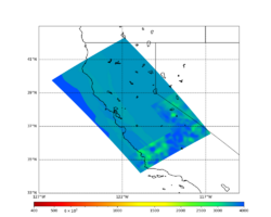
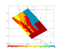
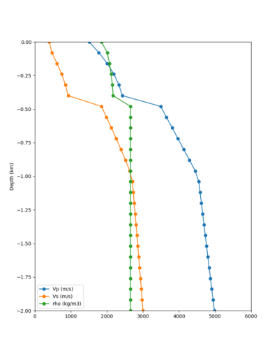
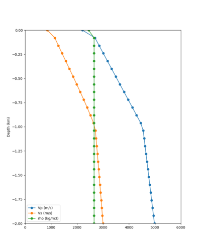
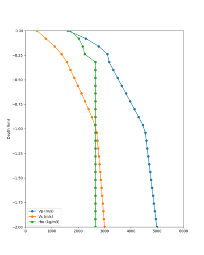
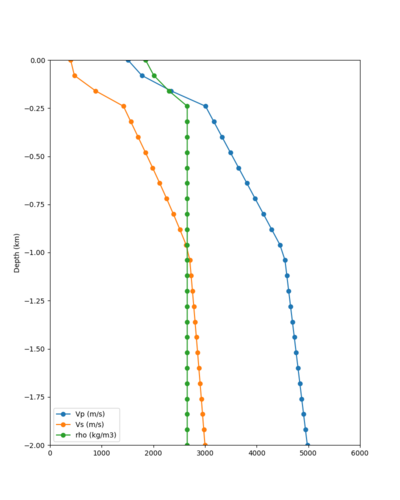
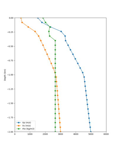
Given the extensive low-velocity near-surface regions in the USGS SF CVM, we plan to use a minimum Vs of 400 m/s (and therefore a grid spacing of 80 m).
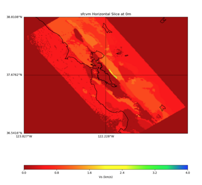
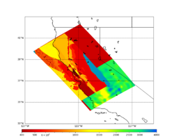
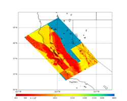
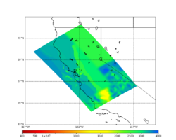
Initial slices with the USGS SF CVM are available here: UCVM_sfcvm_geomodelgrid. We found two sharply defined high-velocity patches visible on the surface slice, one in the East Bay near the mountains, and another near Gilroy. These are regions where the gabbro type goes to the surface, and so the SF CVM geological rules dictate that the high velocities go to the surface as well.
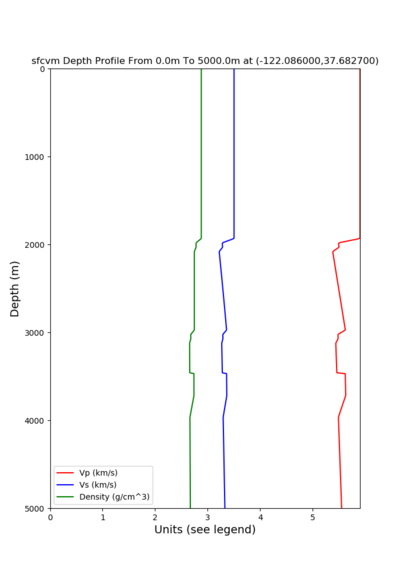
These patches are not present in the Vs30 models - for instance, for the point (37.6827, -122.086) SF CVM gives a surface Vs of about 3500 m/s, but Wills (2015) has Vs30=710 and Thompson (2018) has Vs30=702.
Potential modification to gabbro regions
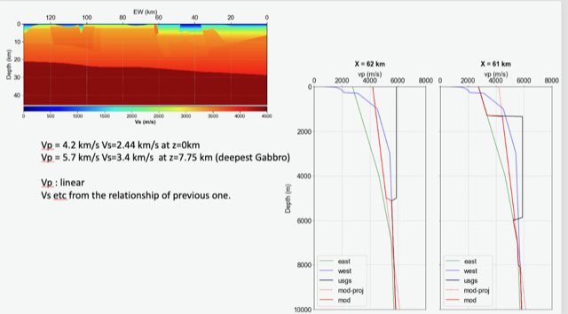
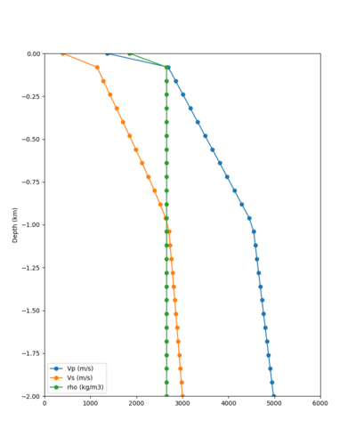
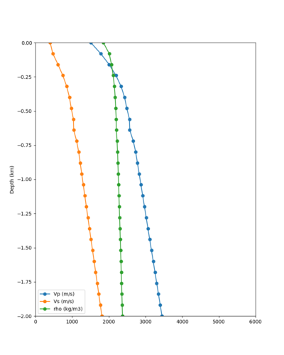
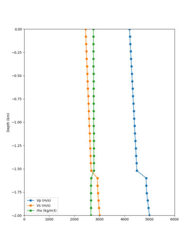
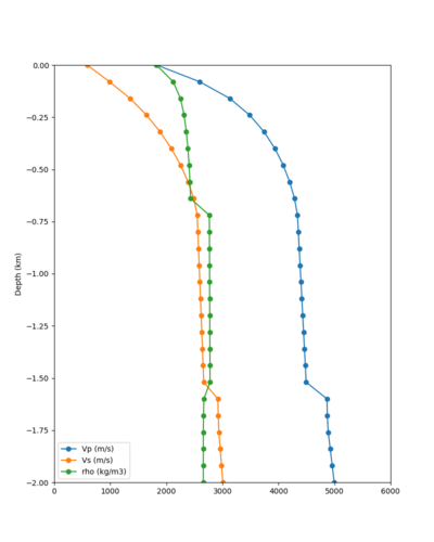
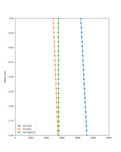
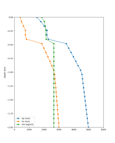
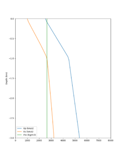
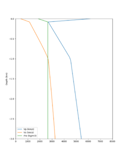
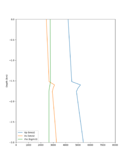
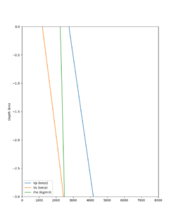
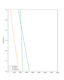
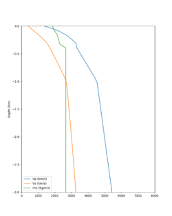
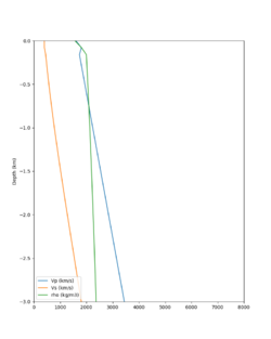
A candidate modification to the gabbro regions to reduce the near-surface velocities is to apply the approach used by Arben Pitarka and Rie Nakata, detailed below.
| Component | At surface | At 7.75 km depth | derivation |
|---|---|---|---|
| Vp | 4.2 km/s | 5.7 km/s | Linear interpolation |
| Vs | 2.44 km/s | 3.4 km/s | Vp/Vs relationship |
| Density | 2.76 g/cm3 | 2.87 g/cm3 | Vp/Density relationship |
The Vs (km/s) values are derived from Vp (km/s) using the San Leandro Gabbro relationship:
Vs = 0.7858 - 1.2344*Vp + 0.7949*Vp^2 - 0.1238*Vp^3 + 0.0064*Vp^4
The density (g/cm3) values are derived from Vp (km/s) using the San Leandro Gabbro relationship:
density = 2.4372 + 0.0761*Vp
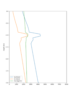
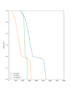
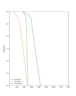
A sample plot is below.
Background model
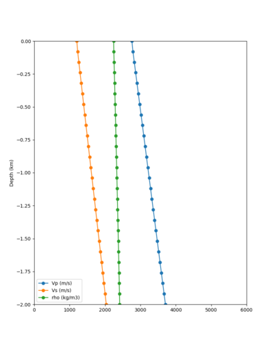
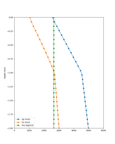
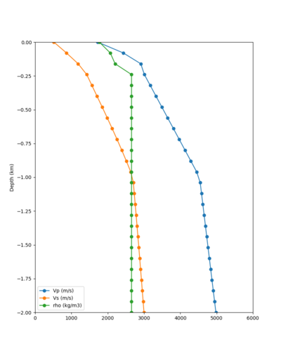
There are several candidates to use as a background model for the regions outside of the 3D model region.
1D models
- 1D Broadband Platform model - either Northern California, Central California, or the Southern Sierras.
- 1D CVM-S4 background model
- Extend eastern edge of SFCVM model to fill the remaining volume
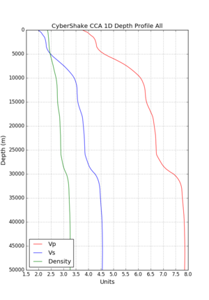
- 1D CCA model (derived from averaging CCA-06), used in Study 17.3
3D models
- 3D CANVAS long-period tomography model
- 3D National Crustal model
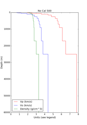
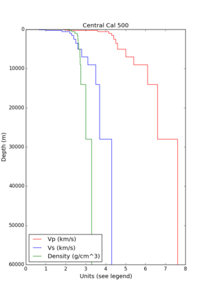
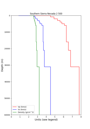
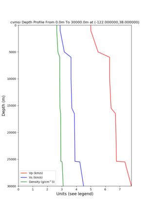
Plots of these options are available below.
| 1D Model | BBP NorCal | BBP CenCal | BBP SouthernSierras | CVM-S4.26.M01 1D background | CCA 1D |
|---|---|---|---|---|---|
| Plot |
Cross-sections
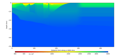
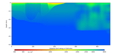
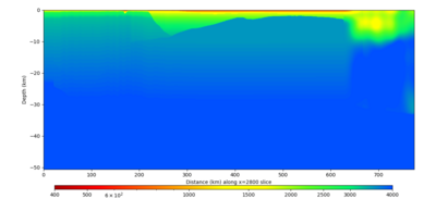
Cross-sections, no smoothing, CVM-S4.26.M01 1D background
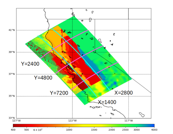
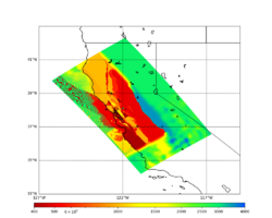
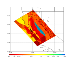
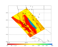
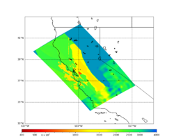
Below are horizontal cross-sections at various depths taken from a model for s3446 generated without smoothing, with the tiling SFCVM, CCA-06, CVM-S4.26.M01. This model was extracted on 2/28/24, and is one of the largest volumes needed for the study.
| 0m | 80m | 800m | 2000m | 4000m | 10000m |
|---|---|---|---|---|---|
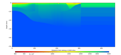
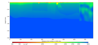
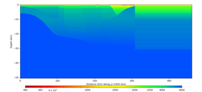
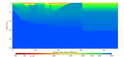
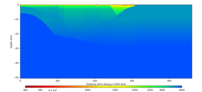
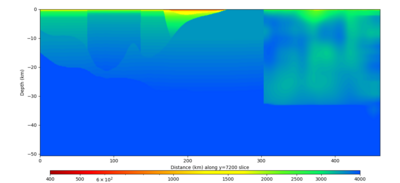
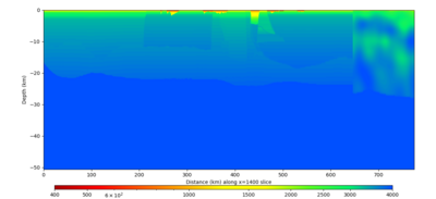
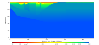
Below are vertical cross-sections taken from a model for s3446 generated without smoothing, with the tiling SFCVM, CCA-06, CVM-S4.26.M01. This model was extracted on 2/28/24, and is one of the largest volumes needed for the study.
| Y=2400 | Y=4800 | Y=7200 |
|---|---|---|
| X=1400 | X=2800 |
|---|---|
Cross-sections, smoothing, CVM-S4.26.M01 1D background
Below are horizontal cross-sections at various depths taken from a model for s3446 generated with smoothing, with the tiling SFCVM, CCA-06, CVM-S4.26.M01. This model was extracted on 2/28/24.
| 0m | 80m | 800m | 2000m | 4000m | 10000m |
|---|---|---|---|---|---|
Below are vertical cross-sections taken from a model for s3446 generated with smoothing, with the tiling SFCVM, CCA-06, CVM-S4.26.M01. This model was extracted on 2/28/24.
| Y=2400 | Y=4800 | Y=7200 |
|---|---|---|
| X=1400 | X=2800 |
|---|---|
Cross-sections, no smoothing, Southern Sierra BBP 1D background
Below are horizontal cross-sections at various depths taken from a model for s3446 generated without smoothing, with the tiling SFCVM, CCA-06, Southern Sierra BBP1D model. This model was extracted on 3/13/24.
| 0m | 80m | 800m | 2000m | 4000m | 10000m |
|---|---|---|---|---|---|
Below are horizontal cross-sections at various depths taken from a model for s3446 generated without smoothing, with the tiling SFCVM, CCA-06, Southern Sierra BBP1D model. This model was extracted on 3/13/24.
| Y=2400 | Y=4800 | Y=7200 |
|---|---|---|
| X=1400 | X=2800 |
|---|---|
Cross-sections, no smoothing, extended SFCVM Sierra 1D background, CCA + taper
Below are horizontal cross-sections at various depths taken from a model for s3446 generated without smoothing, with the tiling SFCVM, CCA-06 + taper, 1D representation of the Sierra foothills in SFCVM. This model was extracted on 4/2/24.
| 0m | 80m | 800m | 2000m | 4000m | 10000m |
|---|---|---|---|---|---|
Below are vertical cross-sections.
| Y=2400 | Y=4800 | Y=7200 |
|---|---|---|
| X=1400 | X=2800 |
|---|---|
Cross-sections, smoothing, extended SFCVM Sierra 1D background, CCA + taper
Below are horizontal cross-sections at various depths taken from a model for s3446 generated with smoothing, with the tiling SFCVM, CCA-06 + taper, 1D representation of the Sierra foothills in SFCVM. This model was extracted on 4/2/24.
| 0m | 80m | 800m | 2000m | 4000m | 10000m |
|---|---|---|---|---|---|
Below are vertical cross-sections.
| Y=2400 | Y=4800 | Y=7200 |
|---|---|---|
| X=1400 | X=2800 |
|---|---|
Cross-sections, no smoothing, extended SFCVM Sierra 1D background with taper, CCA + taper
Below are horizontal cross-sections at various depths taken from a model for s3446 generated without smoothing, with the tiling SFCVM, CCA-06 + taper, 1D representation of the Sierra foothills in SFCVM + taper. This plot includes our typical practice of populating the surface point by querying the models at a depth of grid_spacing/4, or 20m. This model was extracted on 4/9/24.
| Surface (20m) | 80m | 800m | 2000m | 4000m | 10000m |
|---|---|---|---|---|---|
| Y=2400 | Y=4800 | Y=7200 |
|---|---|---|
| X=1400 | X=2800 |
|---|---|
Candidate Model (RC1)
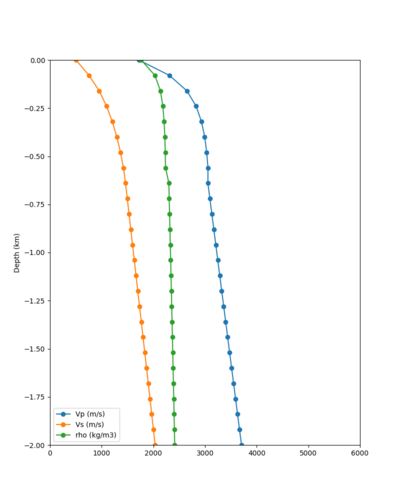
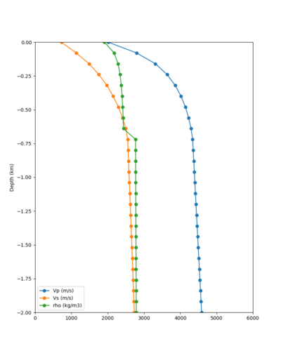
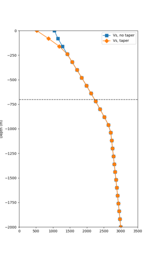
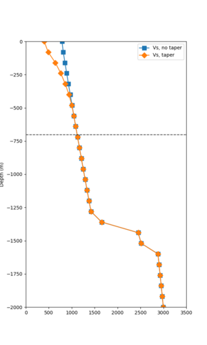
Our candidate model is generated using (1) SFCVM with the gabbro modifications; (2) CCA-06 with the merged taper in the top 700m; (3) the NC1D model with the merged taper in the top 700m.
| Surface (20m) | 80m | 800m | 2000m | 4000m | 10000m |
|---|---|---|---|---|---|
Vp/Vs Ratio Adjustment
For this study, we are modifying our approach to preserving the Vp/Vs ratio when applying a Vs floor to avoid very large Vp/Vs ratios.
Our previous approach for applying the Vs floor is as follows:
- If Vs < Vs_floor (400 m/s):
- Calculate the Vp/Vs ratio
- Change Vs to the floor
- Calculate a new Vp using Vp = Vs_floor * Vp/Vs ratio
- Apply Vp and density floors
However, there are some sites with very high Vp/Vs ratios near the surface where Vs is low. Therefore, if this algorithm is applied, unexpectedly high Vp values may result.
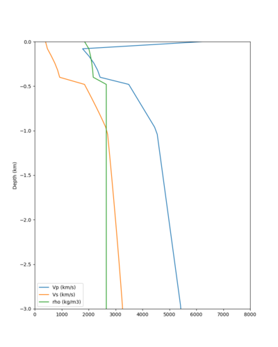
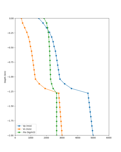
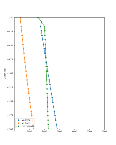
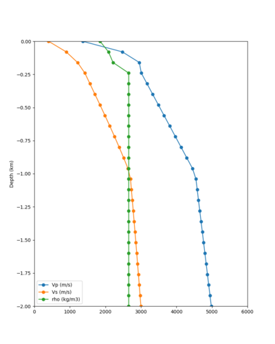
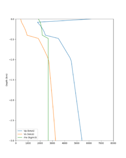
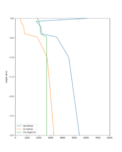
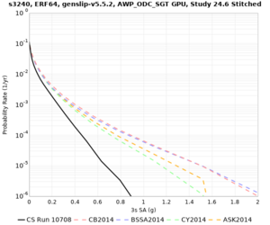
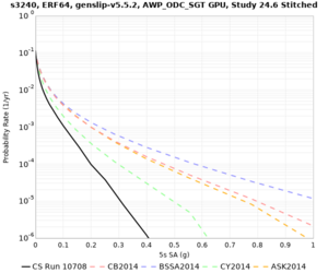
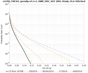
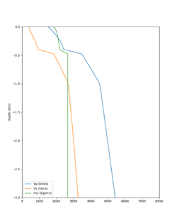
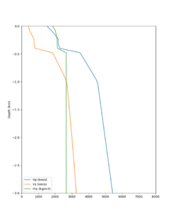
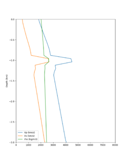
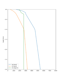
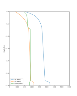
Here is a vertical profile at site s3240 (Moffett Field). You can see the high surface Vp value:
Looking in more detail, here are the Vp and Vs values in the top 90m at s3240:
| Depth (m) | Vp | Vs | Vp/Vs ratio | Adjusted Vs | Adjusted Vp |
|---|---|---|---|---|---|
| 0 | 739 | 81 | 9.12 | 400 | 3649 |
| 10 | 1009 | 82 | 12.30 | 400 | 4922 |
| 20 | 1309 | 84 | 15.58 | 400 | 6233 |
| 30 | 1502 | 152 | 9.88 | 400 | 3953 |
| 40 | 1590 | 285 | 5.58 | 400 | 3649 |
| 50 | 1678 | 418 | 4.01 | ||
| 60 | 1711 | 436 | 3.92 | ||
| 70 | 1744 | 453 | 3.85 | ||
| 80 | 1776 | 471 | 3.77 | ||
| 90 | 1807 | 489 | 3.70 |
Since we are using 80m grid spacing, and populating the surface point at a depth of (grid spacing)/4 = 20m, the values at 20m and 80m are being used. The very high Vp/Vs ratio at 20m means that a very high Vp value is used.
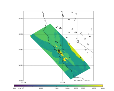
These high Vp/Vs ratios occur at a number of locations around San Francisco Bay, illustrated in the surface Vp plot below:
To solve this problem, we will modify the process for applying the Vs floor. We will use the Vp/Vs ratio at 80m depth instead of at the surface, and use a maximum ratio of 4. A similar process was used in the HighF project.
- If Vs < Vs_floor (400 m/s):
- If surface grid point:
- Calculate Vp/Vs ratio at 1 grid point depth (80m)
- If Vp/Vs ratio > 4:
- Lower Vp/Vs ratio to 4
- Else:
- Calculate Vp/Vs ratio at this grid point
- New Vs = Vs_floor
- New Vp = Vs * (potentially modified) Vp/Vs ratio.
- If surface grid point:
- Apply Vp and density floors.
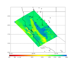
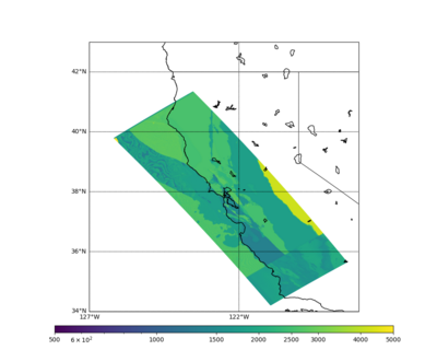
Below is a surface Vp plot with the ratio modification. Note that the areas of previous high Vp have been reduced.
Candidate Model (RC2)
Candidate model RC2 is generated using the following procedure:
- Tiling with:
- USGS SFCVM v21.1
- CCA-06
- 1D background model, derived as an extension of the Sierra section of the SFCVM model and described here.
- Surface points are populated using a depth of (grid spacing)/4, which is 20m for these meshes.
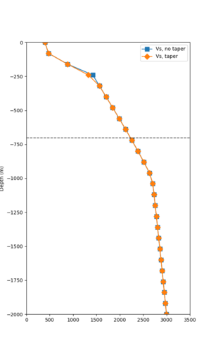
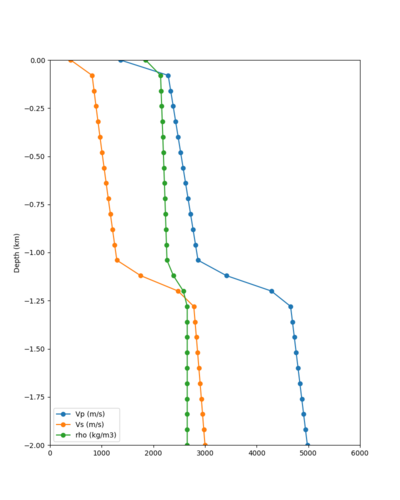
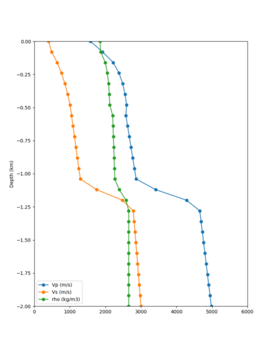
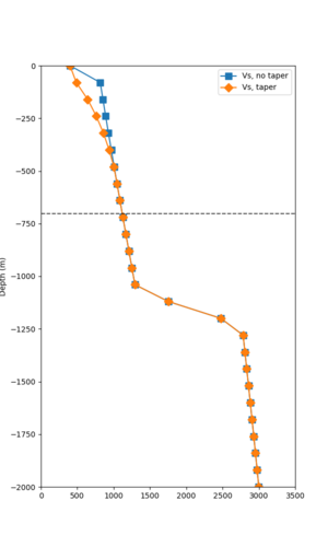
- An Ely-Jordan taper is applied to the top 700m across all models using Vs30 values from Thompson et al. (2020).
- Application of a Vs floor of 400 m/s, using the procedure outlined in CyberShake_Study_24.8#Vp/Vs Ratio Adjustment.
- Smoothing is applied within 20km of a model boundary.
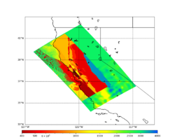
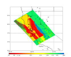
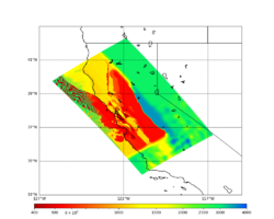
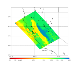
Vs plots:
| Surface (20m) | 80m | 160m | 320m | 640m | 2000m | 4000m | 10000m |
|---|---|---|---|---|---|---|---|
Surface Vp plot:
Taper impact
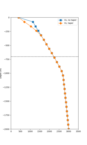
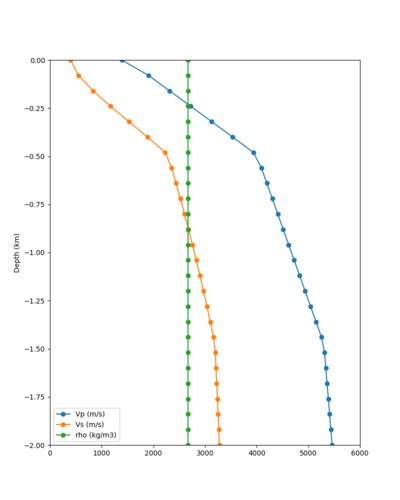
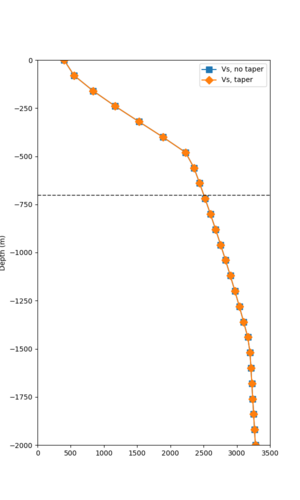
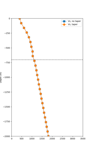
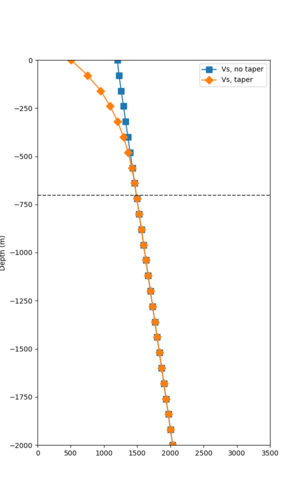
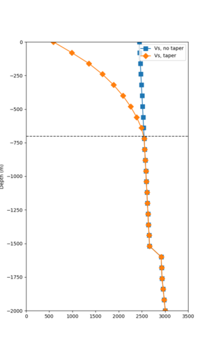
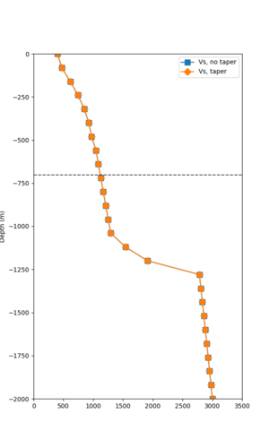
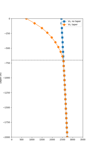
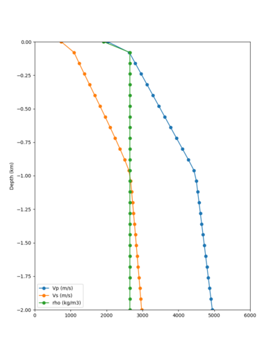
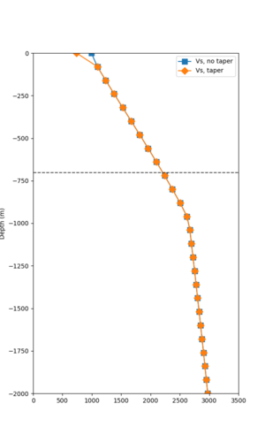
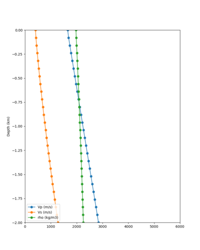
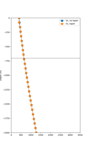
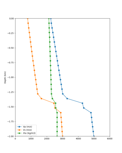
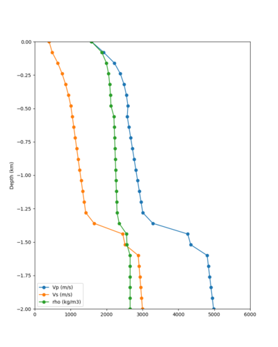
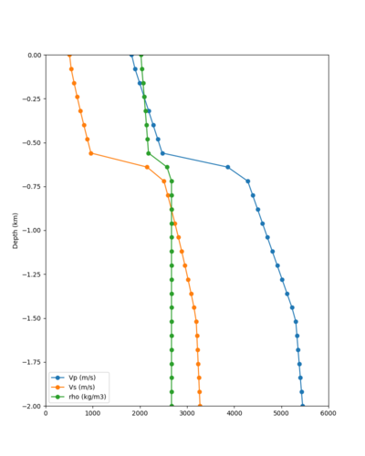
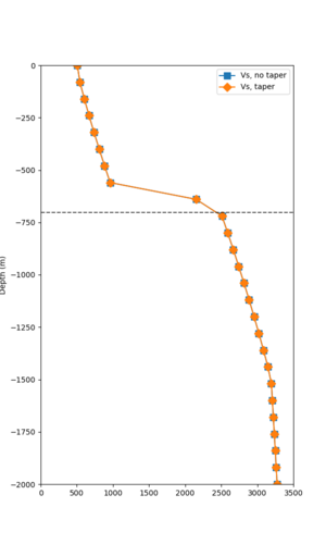
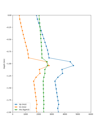
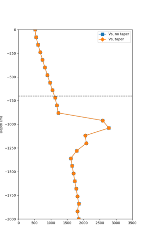
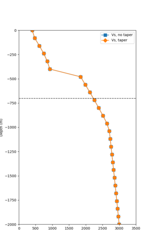
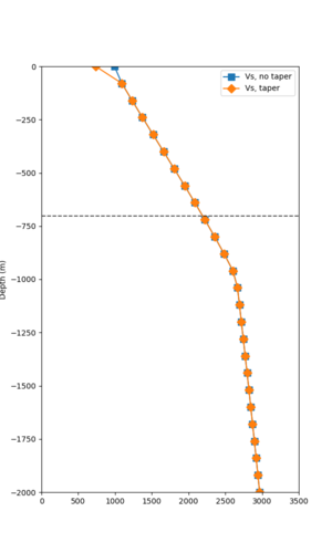
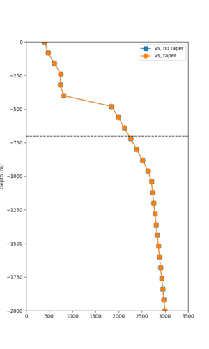
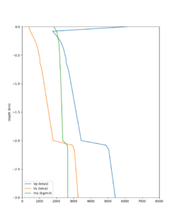
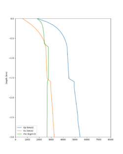
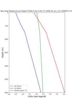
Below are velocity profiles for the 20 stress test sites, with and without the near-surface taper.
| Site | Without taper | With taper (top 700m) | Vs overlay |
|---|---|---|---|
| ALBY | |||
| BLMT | |||
| CFCS | |||
| CSU1 | |||
| CSUEB | |||
| DALY | |||
| HAYW | |||
| LICK | |||
| LVMR | |||
| MSRA | |||
| NAPA | |||
| PTRY | |||
| s3171 | |||
| s3240 | |||
| s3446 | |||
| SFRH | |||
| SSFO | |||
| SSOL | |||
| SRSA | |||
| SJO |
Strain Green Tensors
We will use the HIP implementation of AWP-ODC-SGT, with the following parameters:
- Grid spacing: 80 m
- DT: 0.004 sec
- NT: 50000 timesteps by default, increased to 75000 for sites with any site-to-hypocenter distance greater than 450 km.
- Minimum Vs: 400 m/s
SGTs will be saved with a time decimation of 10, so every 0.04 sec.
Vertical Component
We will include vertical (Z) component seismograms in this study. To support this, we will produce Z-component SGTs and include Z-component synthesis in the post-processing and broadband stages.
Verification that the Z component codes are working correctly is documented at Vertical component verification.
Rupture Generator
We will use the same version of the rupture generator that we used for Study 22.12, v5.5.2.
To match the SGT timestep, SRFs will be generated with dt=0.04s, deterministic seismograms will be output with dt=0.04s, and broadband seismograms will use dt=0.01s.
High-frequency codes
We will use the Graves & Pitarka high-frequency codes from the BBP v22.4.
However, since we are using a denser mesh (80m) and a lower minimum Vs (400 m/s), we will not apply site correction to the low-frequency seismograms before combining. Rob states, You may recall that there is a klugy process we have used to estimate the Vref value based on the Vsmin and grid spacing of the model. But, it has only been applied for the case of h=100 m and Vsmin=500 m/s. What I found here is that estimating Vref using the 80m & 400m/s model is that Vref is almost always less than Vs30 (i.e., Vsite). This means that when the site adjustment is applied, the motions are deamplified. This is why we see such a poor fit for the 3D case when using the estimated Vref values. My conclusion at this point is that if we run the 3D calculation with 80 m grid spacing and Vsmin of 400 m/s (or lower), then we probably do not need to apply any site adjustments.
Hazard Curve Tests
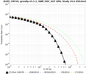
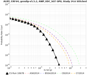
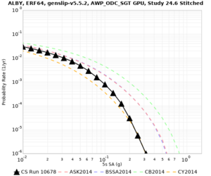
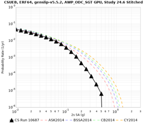
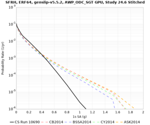
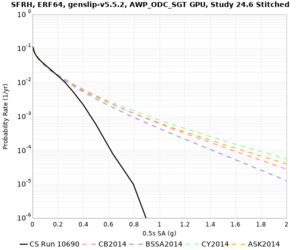
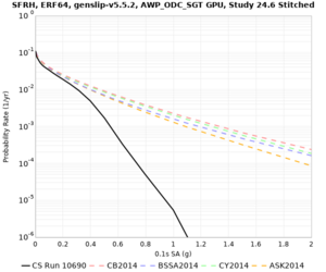
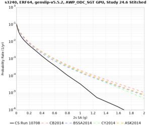
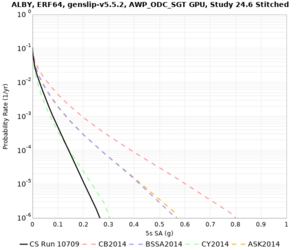
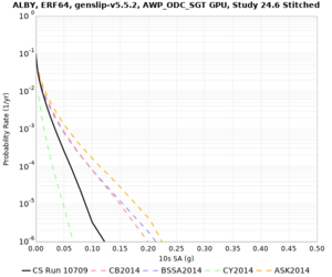
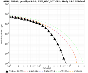
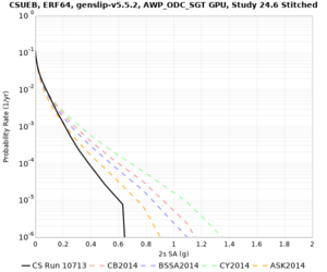
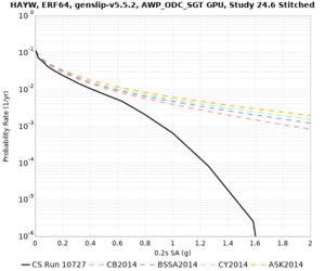
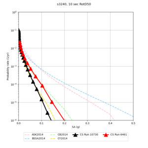
We are calculating test hazard curves for the following sites:
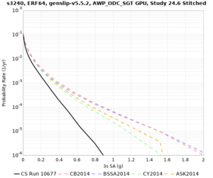
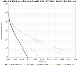
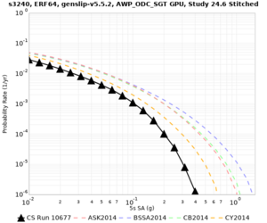
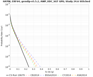
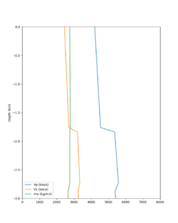
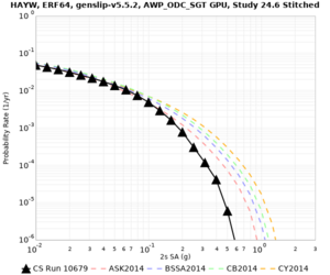
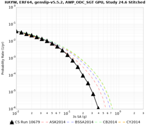
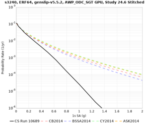
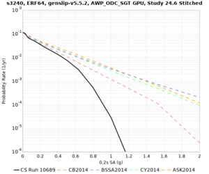
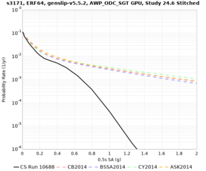
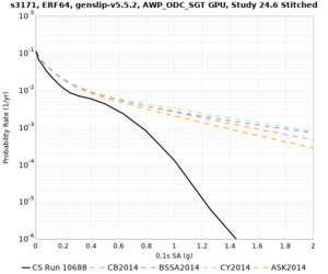
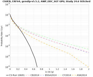
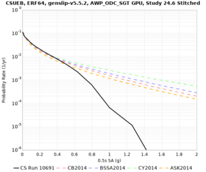
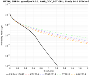
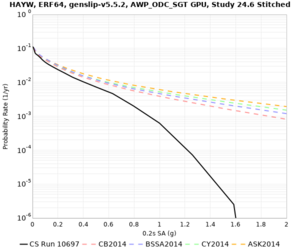
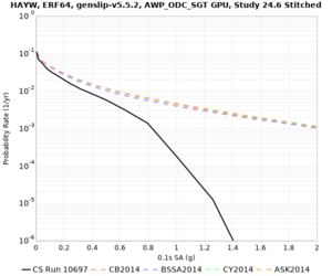
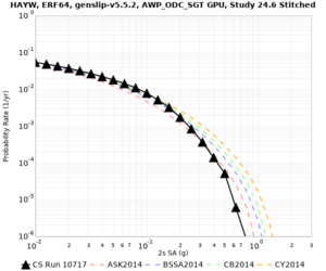
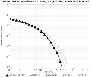
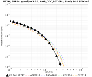
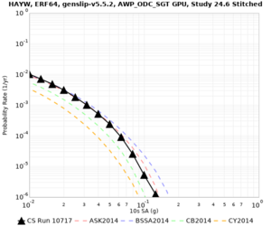
Results using velocity model RC1
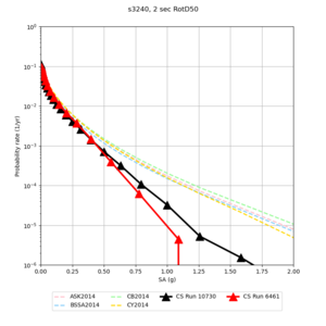
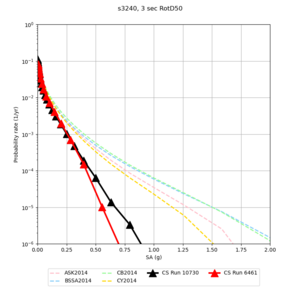
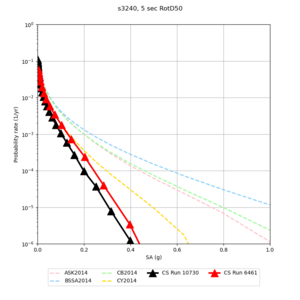
Low-frequency curves
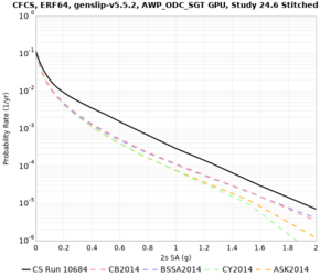
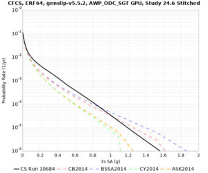
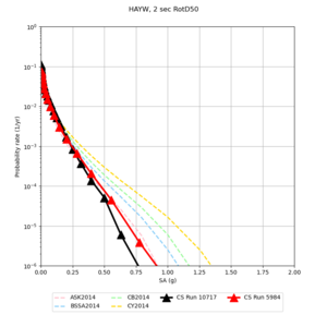
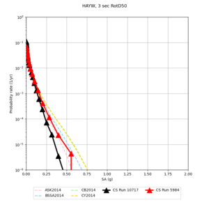
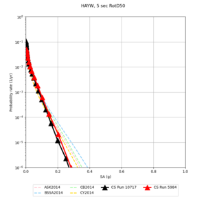
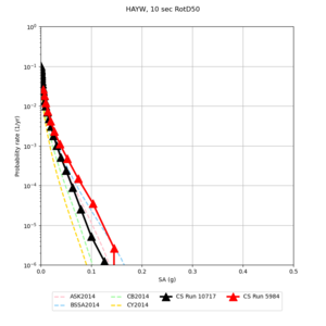
| Site | 2 sec | 3 sec | 5 sec | 10 sec | Vertical profile |
|---|---|---|---|---|---|
| s3446 | |||||
| s3240 | |||||
| ALBY | |||||
| SJO | |||||
| CFCS | |||||
| s3171 | |||||
| CSUEB | |||||
| CSU1 | |||||
| SFRH | |||||
| LVMR | |||||
| HAYW | |||||
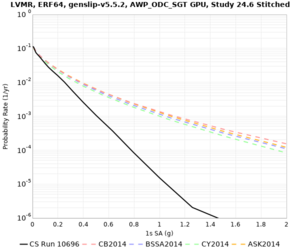
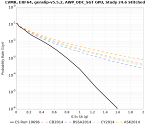
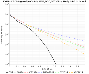
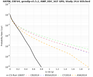
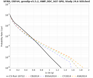
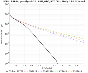
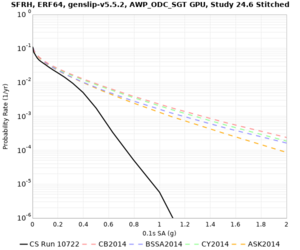
High-frequency curves
| Site | 1 sec | 0.5 sec | 0.2 sec | 0.1 sec | Vertical profile |
|---|---|---|---|---|---|
| s3446 | |||||
| s3240 | |||||
| ALBY | |||||
| SJO | |||||
| CFCS | |||||
| s3171 | |||||
| CSUEB | |||||
| CSU1 | |||||
| SFRH | |||||
| LVMR | |||||
| HAYW |
Results using velocity model RC2
Low-frequency curves
| Site | 2 sec | 3 sec | 5 sec | 10 sec | Vertical profile |
|---|---|---|---|---|---|
| s3240 | |||||
| ALBY | |||||
| SJO | |||||
| CFCS | |||||
| s3171 | |||||
| CSUEB | |||||
| CSU1 | |||||
| SFRH | |||||
| LVMR | |||||
| HAYW | |||||
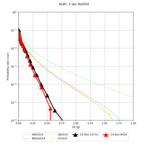
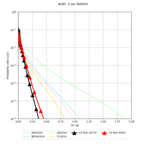
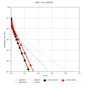
Comparisons with Study 18.8
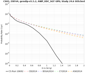
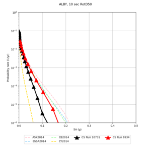
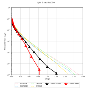
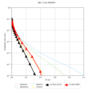
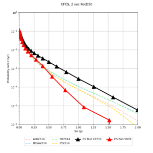
Study 18.8 curves are in red, and new curves are in black.
| Site | 2 sec | 3 sec | 5 sec | 10 sec | Vertical profile |
|---|---|---|---|---|---|
| s3240 | |||||
| ALBY | |||||
| SJO | |||||
| CFCS | |||||
| s3171 | |||||
| CSUEB | |||||
| CSU1 | |||||
| SFRH | |||||
| LVMR | |||||
| HAYW |
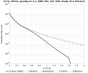
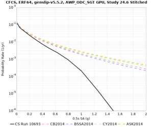
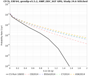
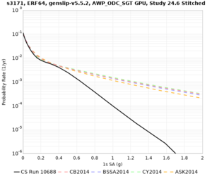
High-frequency curves
| Site | 1 sec | 0.5 sec | 0.2 sec | 0.1 sec | Vertical profile |
|---|---|---|---|---|---|
| s3240 | |||||
| ALBY | |||||
| SJO | |||||
| CFCS | |||||
| s3171 | |||||
| CSUEB | |||||
| CSU1 | |||||
| SFRH | |||||
| LVMR | |||||
| HAYW |
Updates and Enhancements
- Used smaller study region than in Study 18.8.
- Removed southern San Andreas events, and created a new ERF.
Output Data Products
File-based data products
We plan to produce the following data products, which will be stored at CARC:
Deterministic
- Seismograms: 3-component seismograms, 10000 timesteps (400 sec, dt=0.04s) each.
- PSA: We are removing geometric mean PSA calculations from this study.
- RotD: PGV, and RotD50, RotD100, and the RotD100 azimuth at 27 periods (20, 17, 15, 13, 12, 10, 8.5, 7.5, 6.5, 6, 5.5, 5, 4.4, 4, 3.5, 3, 2.8, 2.6, 2.4, 2.2, 2, 1.7, 1.5, 1.3, 1.2, 1.1, 1)
- Vertical response spectra at 27 periods (20, 17, 15, 13, 12, 10, 8.5, 7.5, 6.5, 6, 5.5, 5, 4.4, 4, 3.5, 3, 2.8, 2.6, 2.4, 2.2, 2, 1.7, 1.5, 1.3, 1.2, 1.1, 1).
- Durations: for X and Y components, energy integral, Arias intensity, cumulative absolute velocity (CAV), and for both velocity and acceleration, 5-75%, 5-95%, and 20-80%. Also, period-dependent acceleration 5-75%, 5-95%, and 20-80% for 27 periods (20, 17, 15, 13, 12, 10, 8.5, 7.5, 6.5, 6, 5.5, 5, 4.4, 4, 3.5, 3, 2.8, 2.6, 2.4, 2.2, 2, 1.7, 1.5, 1.3, 1.2, 1.1, 1).
Broadband
- Seismograms: 3-component seismograms, 40000 timesteps (400 sec, dt=0.01s) each.
- PSA: We are removing geometric mean PSA calculations from this study.
- RotD: PGA, PGV, and RotD50, RotD100, and the the RotD100 azimuth at 68 periods (20, 17, 15, 13, 12, 10, 8.5, 7.5, 6.5, 6, 5.5, 5, 4.4, 4, 3.5, 3, 2.8, 2.6, 2.4, 2.2, 2, 1.7, 1.5, 1.3, 1.2, 1.1, 1, 0.85, 0.75, 0.65, 0.6, 0.55, 0.5, 0.45, 0.4, 0.35, 0.3, 0.28, 0.26, 0.24, 0.22, 0.2, 0.17, 0.15, 0.13, 0.12, 0.11, 0.1, 0.085, 0.075, 0.065, 0.06, 0.055, 0.05, 0.045, 0.04, 0.035, 0.032, 0.029, 0.025, 0.022, 0.02, 0.017, 0.015, 0.013, 0.012, 0.011, 0.01)
- Vertical response spectra at 68 periods (20, 17, 15, 13, 12, 10, 8.5, 7.5, 6.5, 6, 5.5, 5, 4.4, 4, 3.5, 3, 2.8, 2.6, 2.4, 2.2, 2, 1.7, 1.5, 1.3, 1.2, 1.1, 1).
- Durations: for X and Y components, energy integral, Arias intensity, cumulative absolute velocity (CAV), and for both velocity and acceleration, 5-75%, 5-95%, and 20-80%. Also, period-dependent acceleration 5-75%, 5-95%, and 20-80% for 68 periods (20, 17, 15, 13, 12, 10, 8.5, 7.5, 6.5, 6, 5.5, 5, 4.4, 4, 3.5, 3, 2.8, 2.6, 2.4, 2.2, 2, 1.7, 1.5, 1.3, 1.2, 1.1, 1, 0.85, 0.75, 0.65, 0.6, 0.55, 0.5, 0.45, 0.4, 0.35, 0.3, 0.28, 0.26, 0.24, 0.22, 0.2, 0.17, 0.15, 0.13, 0.12, 0.11, 0.1, 0.085, 0.075, 0.065, 0.06, 0.055, 0.05, 0.045, 0.04, 0.035, 0.032, 0.029, 0.025, 0.022, 0.02, 0.017, 0.015, 0.013, 0.012, 0.011, 0.01)
Database data products
We plan to store the following data products in the database on moment-carc:
Deterministic
- RotD50 for 6 periods (10, 7.5, 5, 4, 3, 2). Note that we are NOT storing RotD100.
- Duration: acceleration 5-75% and 5-95% for both X and Y
Broadband
- RotD50 for PGA, PGV, and 19 periods (10, 7.5, 5, 4, 3, 2, 1, 0.75, 0.5, 0.4, 0.3, 0.2, 0.1, 0.075, 0.05, 0.04, 0.03, 0.02, 0.01). Note that we are NOT storing RotD100.
Hazard products
For each site, we will produce hazard curves from the deterministic results at 10, 5, 3, and 2 seconds, and from the broadband results at 10, 5, 3, 2, 1, 0.5, 0.2, and 0.1 seconds.
When the study is complete, we will produce maps from the deterministic results at 10, 5, 3, and 2 seconds, and from the broadband results at 10, 5, 3, 2, 1, 0.5, 0.2, and 0.1 seconds.
Data products after the study
After the study completes, we plan to compute Fourier spectra for all 3 components:
- For deterministic, at 27 periods (20, 17, 15, 13, 12, 10, 8.5, 7.5, 6.5, 6, 5.5, 5, 4.4, 4, 3.5, 3, 2.8, 2.6, 2.4, 2.2, 2, 1.7, 1.5, 1.3, 1.2, 1.1, 1).
- For broadband at 68 periods (20, 17, 15, 13, 12, 10, 8.5, 7.5, 6.5, 6, 5.5, 5, 4.4, 4, 3.5, 3, 2.8, 2.6, 2.4, 2.2, 2, 1.7, 1.5, 1.3, 1.2, 1.1, 1, 0.85, 0.75, 0.65, 0.6, 0.55, 0.5, 0.45, 0.4, 0.35, 0.3, 0.28, 0.26, 0.24, 0.22, 0.2, 0.17, 0.15, 0.13, 0.12, 0.11, 0.1, 0.085, 0.075, 0.065, 0.06, 0.055, 0.05, 0.045, 0.04, 0.035, 0.032, 0.029, 0.025, 0.022, 0.02, 0.017, 0.015, 0.013, 0.012, 0.011, 0.01)
Computational and Data Estimates
Computational Estimates
We based these estimates on the test sites.
| UCVM runtime | UCVM nodes | SGT runtime (3 components) | SGT nodes | Other SGT workflow jobs | SGT Total | |
|---|---|---|---|---|---|---|
| Average of 11 test sites | 761 sec | 96 | 7134 sec | 100 | 7200 node-sec | 220 node-hrs |
220 node-hrs/site x 315 sites + 10% overrun = 76,230 node-hours for SGT workflows on Frontier.
| DirectSynth runtime | DirectSynth nodes | Additional runtime for period-dependent calculation | PP Total | |
|---|---|---|---|---|
| 75th percentile of 10 test sites | 13914 sec | 60 | 61938 core-sec | 232.2 node-hrs |
| BB runtime | BB nodes | Additional runtime for period-dependent calculation | BB Total | |
|---|---|---|---|---|
| 75th percentile of 10 test sites | 8019 sec | 40 | 61938 core-sec | 89.4 node-hrs |
(232.2+89.7) node-hrs/site x 315 sites + 10% overrun = 111,500 node-hours for PP and BB calculations on Frontera.
Data Estimates
We use the 75th percentile estimate of 206,500 rupture variations.
We are generating 3-component SGTs and 3-component seismograms, with 10k timesteps (400 sec) for LF and 40k timesteps (400 sec) for BB.
| Velocity mesh | SGTs size | Temp data | LF Output data | BB Output data | Total output data | |
|---|---|---|---|---|---|---|
| Per site, derived from 10 site average (GB) | 359 | 1131 | 1490 | 23.7 | 93.6 | 117.3 |
| Total for 335 sites (TB) | 110 | 348 | 458 | 7.3 | 28.8 | 36.1 |
CARC
We estimate 117.3 GB/site x 315 sites = 36.1 TB in output data, which will be transferred back to CARC. We currently have 29 TB free.
shock-carc
We estimate (3 MB SGT + 32 MB PP + 219 MB BB logs + 3 MB output products) x 315 sites = 79 GB in workflow log space on /home/shock. This drive has approximately 1.2 TB free.
moment-carc database
The PeakAmplitudes table uses approximately 183 bytes for data + 179 bytes for index = 363 bytes per entry.
362 bytes/entry * 35 entries/event (10 det + 25 stoch) * 206,500 events/site * 315 sites = 768 GB. The drive on moment-carc with the mysql database has 6.6 TB free.
Lessons Learned
Stress Test
For the stress test, we will run the first 20 sites and check for scientific and technical issues.
Usage before the stress test:
- On Frontier, 587,856 of 700,000 node-hours for project GEO156. callag has used 22,166 node-hours.
- On Frontera, 316,715 of 600,000 node-hours for project EAR20006. scottcal has used 11,274 node-hours.
The stress test began on 8/27/24 at 11:25:23 PDT.
To help us finish the stress test before the SCEC AM, TACC granted us a Frontera reservation for 200 nodes for 8 days, beginning on 8/28/24 at 8 am PDT. We didn't realized we needed to specify the --reservation tag, so we began utilizing it around 9 am PDT.
We gave the reservation back in the morning of 8/30. After the stress test, callag had used 32,660 node-hours on Frontier and scottcal used 18,493 node-hours on Frontera.
Stress test computational cost:
- SGTs: 10494/20 sites = 524.7 node-hours per site, about 2.4x what we estimated. This is mostly due to having used meshes with a -55 degree angle, resulting in larger meshes requiring more computation time.
- PP and BB: 370.0 node-hours per site, about 15% more than we estimated.
Changes from stress test
Based on the stress test, we made the following changes:
- Reduced ramp-up time for DirectSynth worker processes.
- Fixed issue with PGV writing to files in the BB codes.
- Changed mesh angle from -55 to -36 degrees.
- Changed smoothing zone from 10 km on either side of the boundary to 20 km.
- Fixed issue with vertical response and period duration files not automatically transferred.
- Discovered issue with accessing moment-carc through the USC VPN - confirmed that neither Xiaofeng nor Kevin can access it.
Stress test results
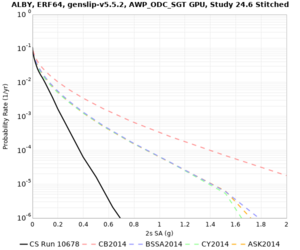
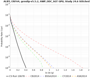
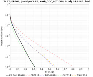
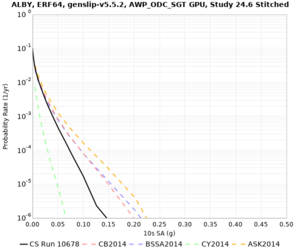
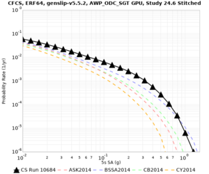
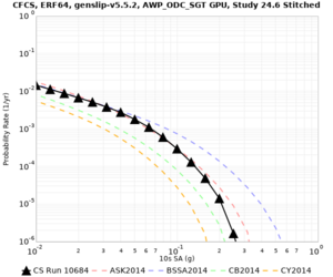
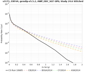
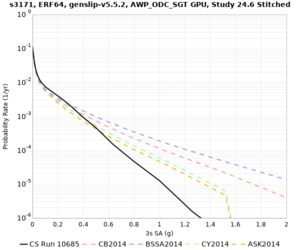
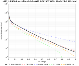
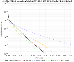
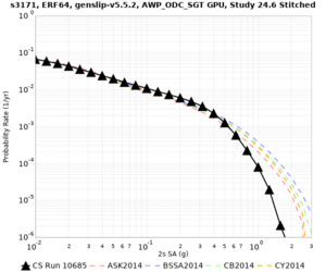
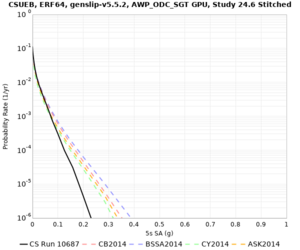
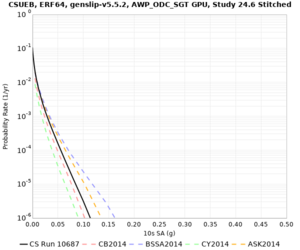
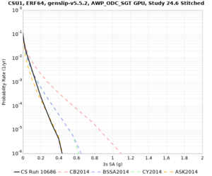
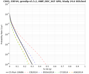
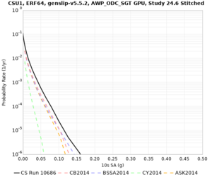
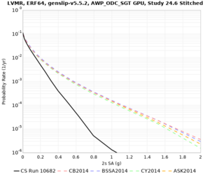
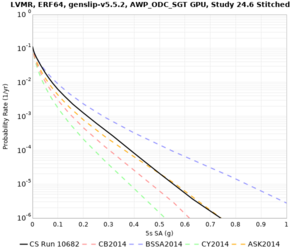
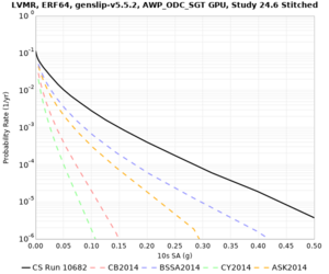
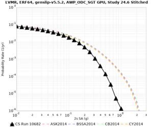
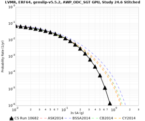
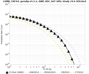
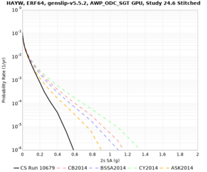
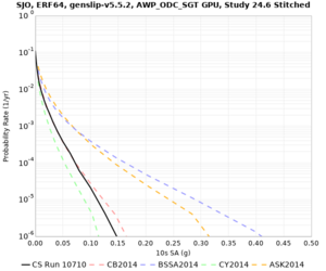
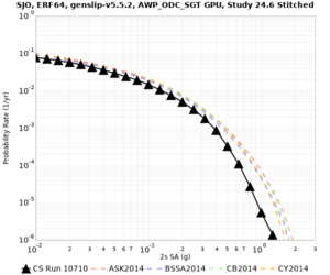
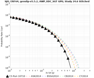
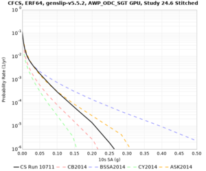
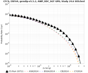
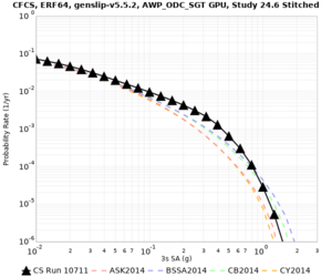
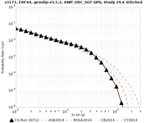
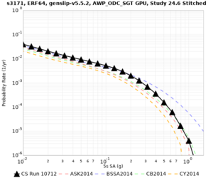
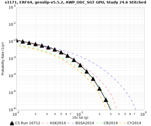
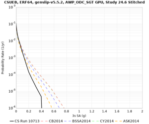
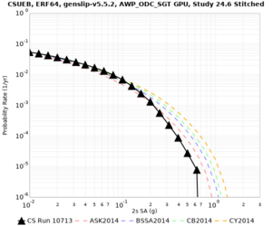
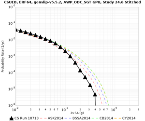
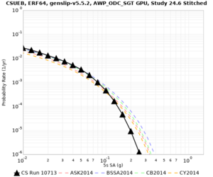
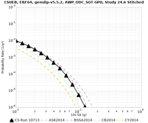
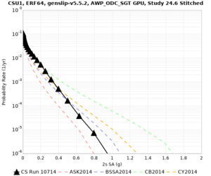
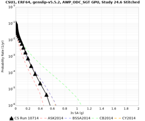
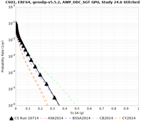
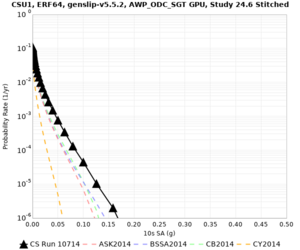
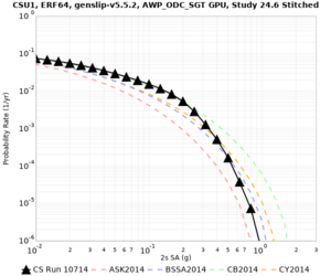
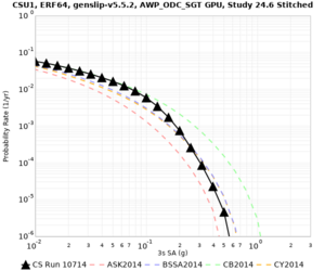
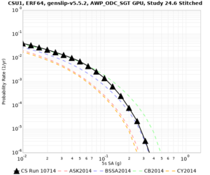
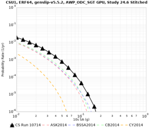
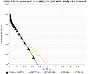
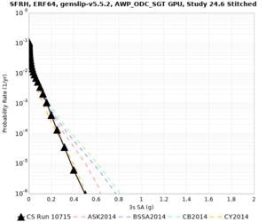
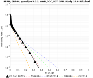
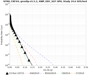
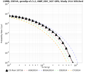
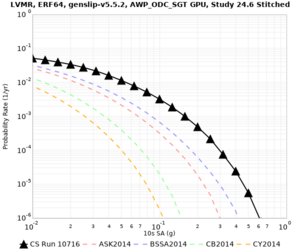
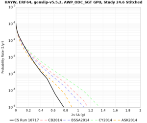
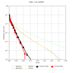
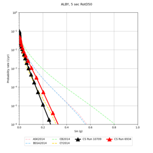
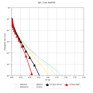
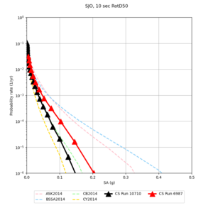
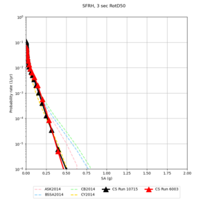
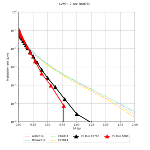
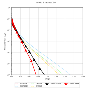
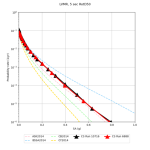
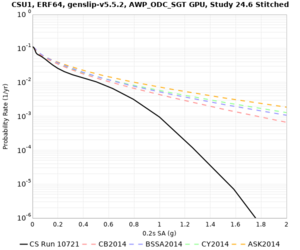
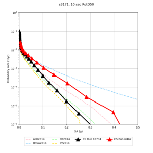
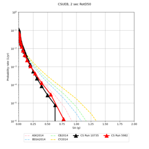
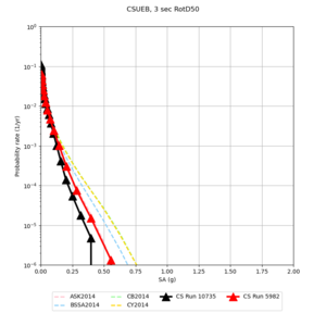
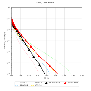
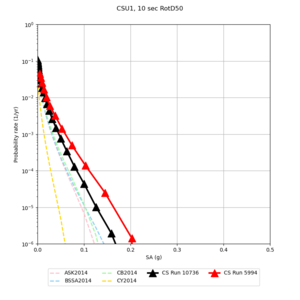
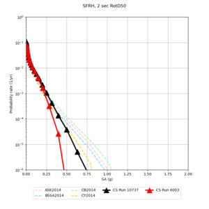
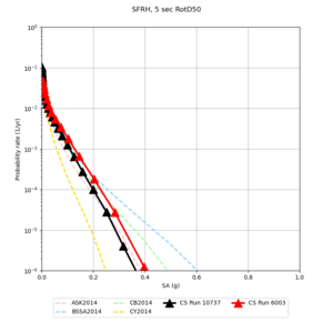
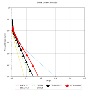
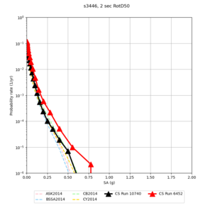
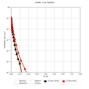
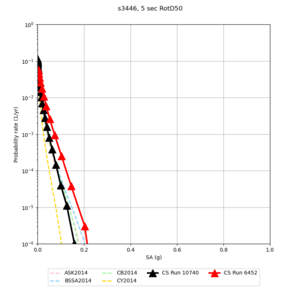
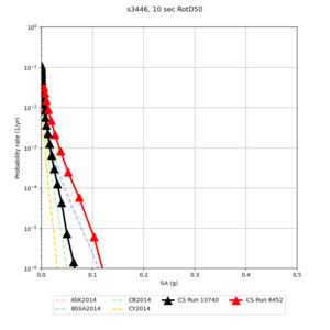
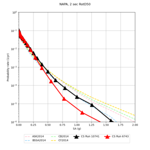
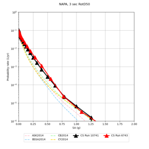
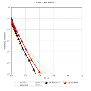
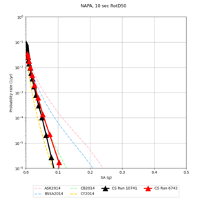
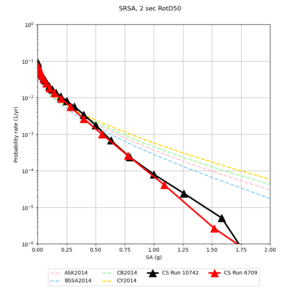
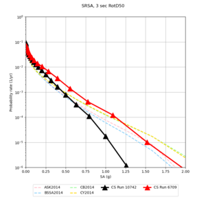
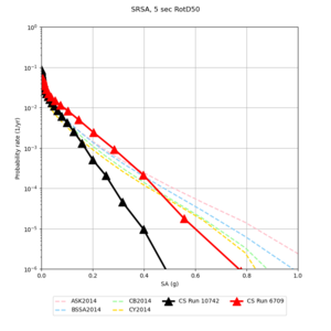
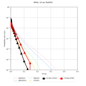
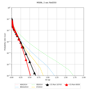
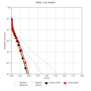
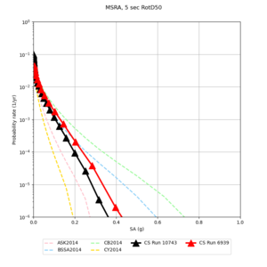
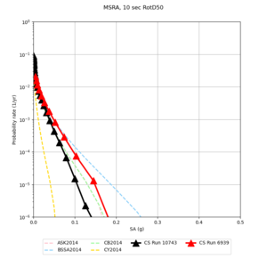
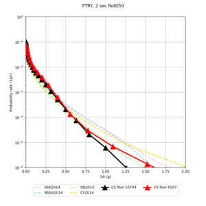
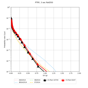
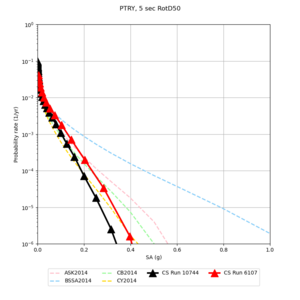
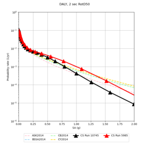
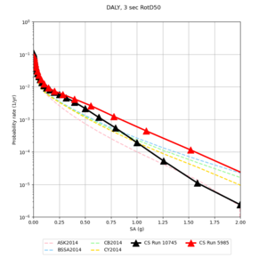
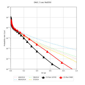
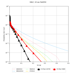
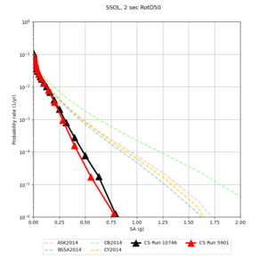
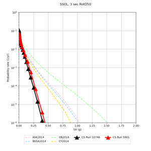
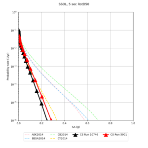
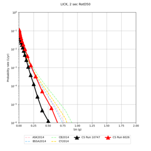
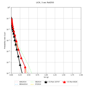
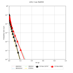
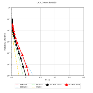
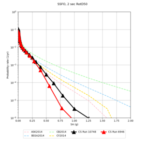
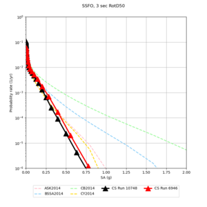
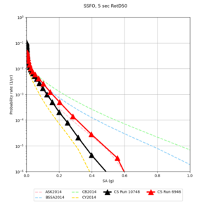
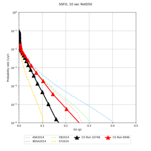
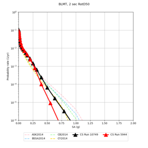
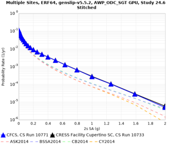
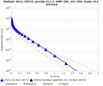
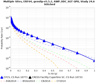
Below are hazard curves for the 20 test sites in the stress test.
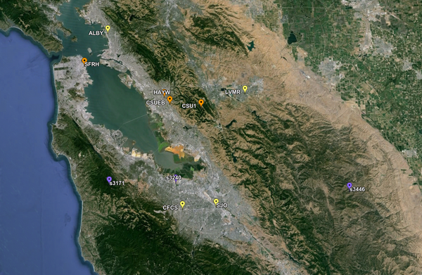
A KML file with the stress test sites is available here.
Low-frequency
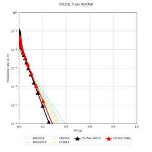
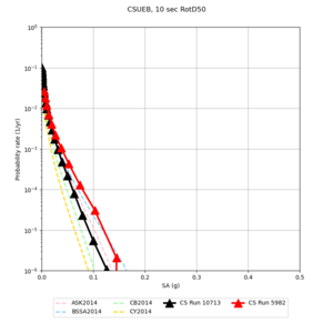
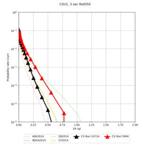
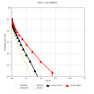
These curves (in black) include comparisons with Study 18.8 (in red)
| Site | 2 sec | 3 sec | 5 sec | 10 sec |
|---|---|---|---|---|
| s3240 | ||||
| ALBY | ||||
| SJO | ||||
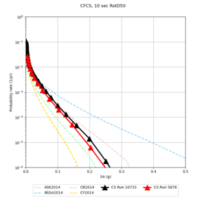
| CFCS | ||||
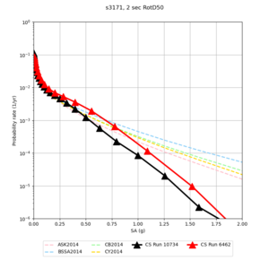
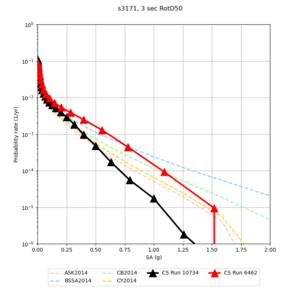
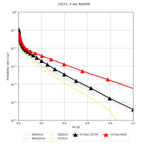
| s3171 | ||||
| CSUEB | ||||
| CSU1 | ||||
| SFRH | ||||
| LVMR | ||||
| HAYW | ||||
| s3446 | ||||
| NAPA | ||||
| SRSA | ||||
| MSRA | ||||
| PTRY | ||||
| DALY | ||||
| SSOL | ||||
| LICK | ||||
| SSFO | ||||
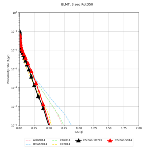
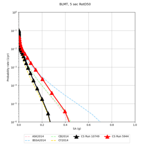
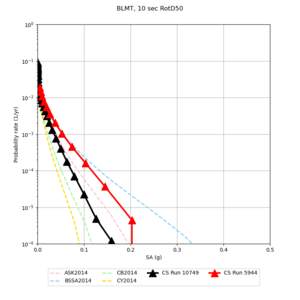
| BLMT |
Sites with notable differences
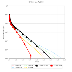
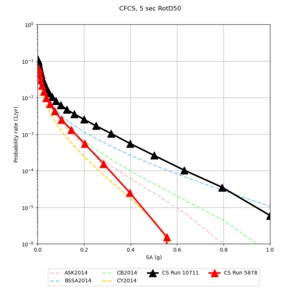
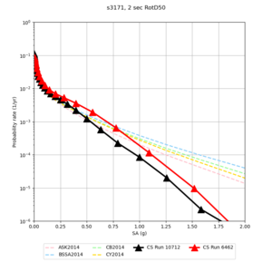
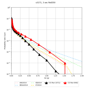
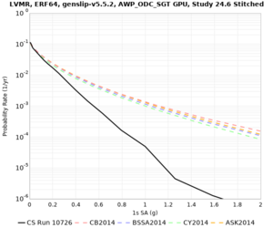
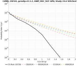
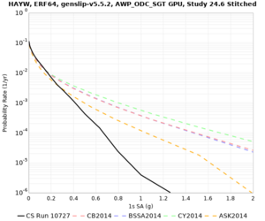
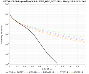
We identified 3 sites with notable differences between Study 24.8 and Study 18.8:
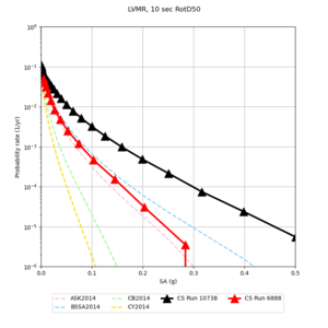
- LVMR is higher at 10 sec
- CFCS is higher 2, 3, 5 sec
- s3171 is lower at 3, 5, 10 sec
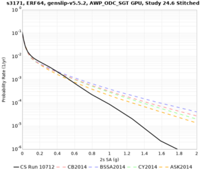
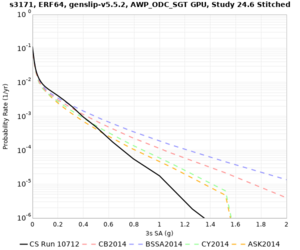
We believe the difference in LVMR is due to the expanded basin added in SFCVM v21.1, and s3171 can be explained by the change in profile as well:
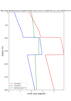
| Site | Profile, SFCVM v21.1 | Profile, Cencal model used in Study 18.8 |
|---|---|---|
| LVMR | ||
| s3171 |
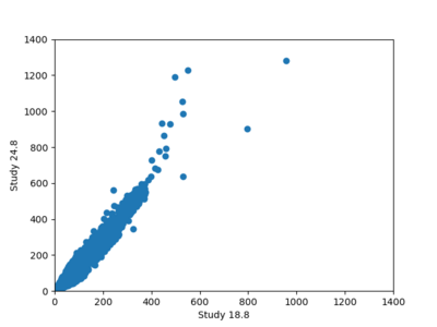
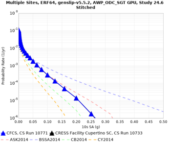
A scatterplot comparing the average 2 sec RotD50 value for each rupture shows that the Study 24.8 results are consistently higher than the 18.8 results for CFCS:
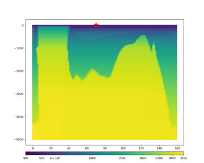
We extracted vertical slices for the top from Cencal (floor = 500 m/s) and the Study 24.8 model (taper, floor = 400 m/s) for the top 5000 m along an east-west line running through CFCS.
| Vertical slice, Study 24.8 | Vertical slice, Cencal |
|---|---|
Corrected Study 18.8 comparisons
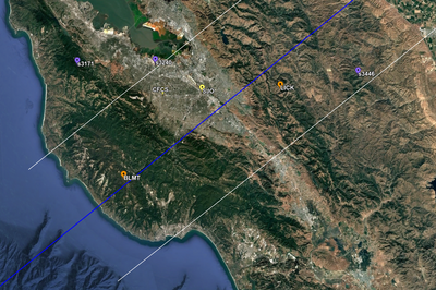
In an attempt to replicate the Study 18.8 results, we discovered that the Study 18.8 velocity models were tiled in a different order than for Study 24.8: CCA-06, then CenCal, then CVM-S4.26.M01, as described here. Several of the stress test sites fall within the 20 km smoothing zone surrounding the Study 18.8 CCA-06/Cencal interface (interface in blue, 20km zone in white):
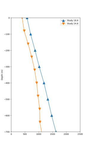
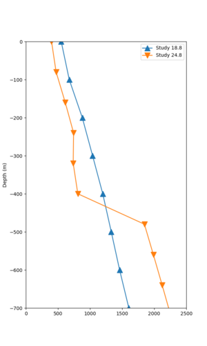
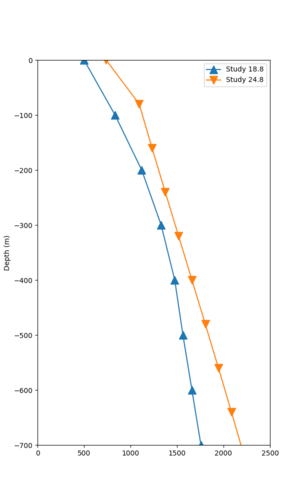
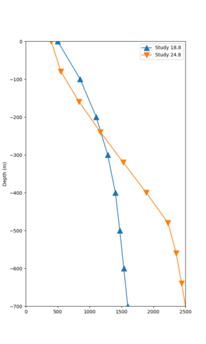
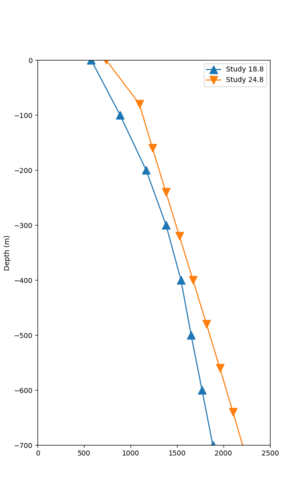
We compared the velocity profiles of Study 24.8 and the correct Study 18.8 configuration for the 5 stress test sites. For CFCS, this explains the sharp increase in hazard. The Study 18.8 profile is in blue, and the Study 24.8 profile is in orange.
| Site | Vs overlay, top 700m | 2 sec curve | 3 sec curve | 5 sec curve | 10 sec curve |
|---|---|---|---|---|---|
| CFCS | |||||
| SJO | |||||
| s3446 | |||||
| BLMT | |||||
| LICK |
Impact of rotation angle and smoothing zone
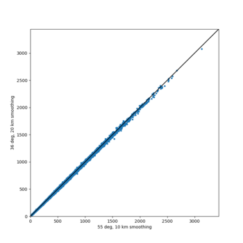
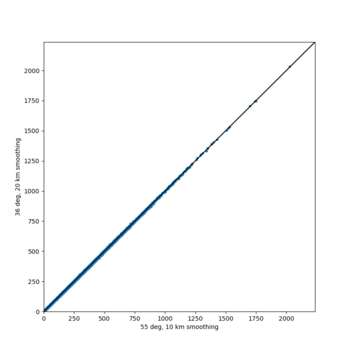
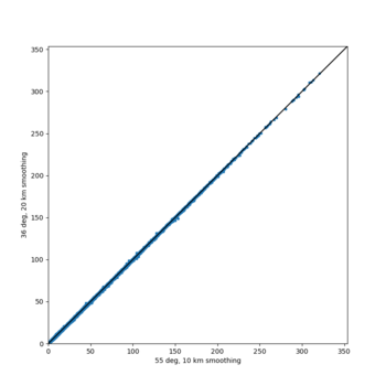
Based on the below analysis, we will rerun the stress test sites with the intended angle of -36 degrees and a 20 km smoothing zone so that all Study 24.8 results will be consistent.
We discovered that the stress test sites were run with a volume rotation angle of -55 degrees and a smoothing zone width of 10 km on either side of the interface. This is different from our intended rotation angle of -36 degrees and smoothing zone width of 20 km. To quantify the impact of this, we ran CFCS with the updated values. Comparisons are below. The black curves are the stress test run, the blue curves are the corrected run.
| 2 sec | 3 sec | 5 sec | 10 sec |
|---|---|---|---|
Events During Study
The main study began on 9/24/24 at 11:49:59 PDT.
We began with a maximum of 5 workflows on Frontier and 20 on Frontera. Later on 9/24 we increased the number of Frontier workflows to 15.
On 9/30, moment-carc wasn't passed to the Check Duration job for finishing PP workflows. I updated the dax generator to correctly pass through the desired database for this job.
On 9/30, I ran out of /home quota on Frontera. This was an issue because some of the rvGAHP-related logs are written here, and it resulted in "Failed to start transfer GAHP" errors. I cleaned up some space on /home and released the jobs.
On 9/30, the merge_pmc jobs were held because they still included the stress test reservation on Frontera. I removed the reservation string and released the jobs.
On 10/1, I found that the cronjob on Frontier to monitor job usage was removed from the crontab, so I added it back.
On 10/2, I turned off stochastic calculations on Frontera while we investigated the unexpected BB results from the stress test.
On 10/10, the work2 filesystem on Frontera, where the executables and rupture files are hosted, had a problem, causing all the Frontera jobs to be held. Additionally, login4, the host which connects to shock, was unavailable. When login4 returned we restarted the rvGAHP process.
On 10/16, the scottcal account was added to the CyberShake DesignSafe project. This meant that scottcal is now part of 3 allocations, leading to a Slurm error when jobs were submitted without specifying an account, meaning Condor jobs were held. I added the EAR20006 account to all Frontera jobs, and had to manually add it for jobs which were already planned.
On 10/16, I realized that DirectSynth jobs were requesting a wallclock time of 10 hours, but these jobs are usually only taking a bit more than 4. I changed the requested job length to 5 hours.
On 10/17, I discovered that the PP Error jobs were because the corresponding SGT workflow had finished its Update and Handoff jobs, but then the stage-out of the SGTs to Frontera failed because of Globus consents. The registration job is dependent on stage-out, so it didn't run either. Then, when the PP workflow tries to plan, it can't find a copy of the SGT files on Frontera and aborts. I couldn't use the standard CyberShake scripts to restart these workflows, since in the database they were already recorded as SGT Generated, so instead I just reran the pegasus-run commands in the log-plan* files.
On 10/18, I got an email from TACC staff that the jobs are causing too much load on the scratch filesystem, and a request to reduce the number of simultaneous jobs to 4. I reduced the number of Frontera slots to 4 in the workflow auto-submission tool, and am following up to learn the specifics of the problem and if there's a way to fix it.
SGT calculations on Frontier finished on 10/18/24 at 12:59:43 PDT.
On 10/21, the broadband transfers to Corral for Study 22.12 resulted in going over quota on CARC scratch1 again, interfering with the workflows for this study. I cleaned up scratch1 and fixed the issue.
On 10/28-30, the work2 filesystem and scheduler on Frontera had a number of issues, requiring restarts of the rvGAHP daemon and some work to recover the job state.
Renewal of Globus consents
We will track when we renew the Globus consents.
10/6
10/9
10/13
10/17
10/24
10/29
11/5
Restarts of the rvgahp daemons
We will track when we restart the rvgahp daemons on login10@frontier and login4@frontera.
10/9 on Frontera
10/10 on Frontera (node crashed)
10/29 on Frontera (filesystem issues)
10/30 on Frontera (continuing filesystem issues)
11/7 on Frontera
Performance Metrics
At the start of the main study, project geo156 on Frontier has used 609101 node-hours (of 700,000). User callag has used 33398 node-hours. Project EAR20006 has used 12925.147 node-hours (of 676,000). User scottcal has used 503.796 node-hours.
At the end of the main study, project geo156 had used 671,656 node-hours. User callag has used 88881.2 node-hours. project EAR20006 had 511480 node-hours remaining (out of 676,000). User scottcal used 125411.21 node-hours.
In total, the study used 55483 node-hours on Frontier and 124907 node-hours on Frontera.
Our high-water marks were 4130 nodes on Frontier (44%) and 1029 nodes on Frontera (12%). Neither used a reservation or priority bump.
Pegasus managed about 1 PB of data.
We staged about 9 million output files totaling 36 TB back to long-term storage at USC CARC.
We ran 945 top-level workflows, with an average of 15 running at a time.
We ran approximately 27,720 jobs. Of these, 7245 were remote, 8190 were local, 5985 were directory creation, 5355 were staging, and 945 were registration.
126,818,608 three-component seismograms (half LF, half BB), 11.5 billion low-frequency IMs, and 22.8 billion broadband IMs were calculated.
Production Checklist
Run test workflow against moment-carc.Investigate velocity profile differences with Mei's plots (s3171 and HAYW)Wrap period-dependent duration code and test in PP.Wrap period-dependent duration code and test in BB.Integrate period-dependent duration code into workflows.Update data and compute estimates.Determine where to copy output data.Modify workflows to remove double-staging of SGTs to Frontera.Schedule and hold readiness reviews with TACC and OLCF.Modify workflows to only insert RotD50, not RotD100.Science readiness reviewTechnical readiness reviewVerify that vertical component response is being calculated correctly.Set up cronjobs to monitor usage.Solve issue with putting velocity parameters into the database from Frontier.Tag code in github repository
