Difference between revisions of "CyberShake Study 18.8"
| Line 195: | Line 195: | ||
== Alternative Velocity Model Plots == | == Alternative Velocity Model Plots == | ||
| − | |||
| − | |||
| − | + | The following plots represent a proposed Northern California Velocity Model. Create using an updated version of the UCVM Software: The tiling order of velocity models in these plots is: | |
| − | + | ||
| − | + | Science Name (ucvmc abbreviation): | |
| − | + | #USGS Bay Area Model (cencal) | |
| − | + | #CCA06 (cca) | |
| − | + | #CVM-S4.26 (cvms5) | |
| − | + | #Modified Hadley Kanamori 1D (1d) | |
| − | + | Tiled without adding Ely-Jordan GTL to CCA06 or CVM-S4.26 | |
{| | {| | ||
| [[File:cross_study_no_depth_0.png|thumb|300px|0 km depth]] | | [[File:cross_study_no_depth_0.png|thumb|300px|0 km depth]] | ||
| Line 214: | Line 212: | ||
|} | |} | ||
| + | Tiled with Ely-Jordan Vs30-based GTL added to CCA06, and CVM-S4.16 | ||
| + | {| | ||
| + | | [[File:cross_study_depth_0.png|thumb|300px|0 km depth]] | ||
| + | | [[File:cross_study_depth_100.png|thumb|300px|0.1 km depth]] | ||
| + | | [[File:cross_study_depth_1000.png|thumb|300px|1 km depth]] | ||
| + | | [[File:cross_study_depth_10000.png|thumb|300px|10 km depth]] | ||
| + | |} | ||
| + | |||
| + | Tiled with Ely-Jordan Vs30-based GTL added to CCA06 and CVM-S4.26 | ||
{| | {| | ||
| [[File:study_cross_x_1500.png|thumb|300px|x index=1500]] | | [[File:study_cross_x_1500.png|thumb|300px|x index=1500]] | ||
| Line 226: | Line 233: | ||
| [[File:study_cross_y_9600.png|thumb|250px|y index=9600]] | | [[File:study_cross_y_9600.png|thumb|250px|y index=9600]] | ||
|} | |} | ||
| − | |||
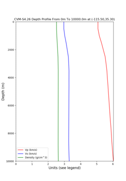
== Depth profiles of 2 selected points: == | == Depth profiles of 2 selected points: == | ||
Revision as of 03:54, 11 April 2018
CyberShake 18.3 is a computational study to perform CyberShake in a new region, the extended Bay Area. We plan to use a combination of 3D models (USGS Bay Area detailed and regional, CVM-S4.26.M01, CCA-06) with a minimum Vs of 500 m/s and a frequency of 1 Hz. We will use the GPU implementation of AWP-ODC-SGT, the Graves & Pitarka (2014) rupture variations with 200m spacing and uniform hypocenters, and the UCERF2 ERF. The SGT and post-processing calculations will both be run on both NCSA Blue Waters and OLCF Titan.
Contents
- 1 Status
- 2 Science Goals
- 3 Technical Goals
- 4 Sites
- 5 Projection Analysis
- 6 Velocity Models
- 7 Updated Vs cross-sections
- 8 Vs cross-sections
- 9 Verification
- 10 Performance Enhancements (over Study 17.3)
- 11 Computational and Data Estimates
- 12 Alternative Velocity Model Plots
- 13 Depth profiles of 2 selected points:
- 14 Production Checklist
- 15 Presentations, Posters, and Papers
- 16 Related Entries
Status
This study is under development. We hope to begin in March 2018.
Science Goals
The science goals for this study are:
- Expand CyberShake to the Bay Area.
- Calculate CyberShake results with the USGS Bay Area velocity model as the primary model.
Technical Goals
- Perform the largest CyberShake study to date.
Sites
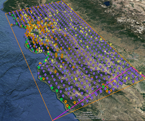
The Study 18.3 box is 180 x 390 km, with the long edge rotated 27 degrees counter-clockwise from vertical. The corners are defined to be:
South: (-121.51,35.52)
West: (-123.48,38.66)
North: (-121.62,39.39)
East: (-119.71,36.22)
We are planning to run 869 sites, 838 of which are new, as part of this study.
These sites include:
- 77 cities (74 new)
- 10 new missions
- 139 CISN stations (136 new)
- 46 new sites of interest to PG&E
- 597 sites along a 10 km grid (571 new)
Of these sites, 32 overlap with the Study 17.3 region for verification.
A KML file with all these sites is available with names or without names.
Projection Analysis
As our simulation region gets larger, we needed to review the impact of the projection we are using for the simulations. An analysis of the impact of various projections by R. Graves is summarized in this posting:
Velocity Models
For Study 18.3, the first velocity model, we examined was the following order of precedence:
- USGS Bay Area model
- CCA-06
- CVM-S4.26.M01 which include a 1D background model
We will apply a minimum Vs of 500 m/s. We will smooth to a distance of 10 km either side of a velocity model interface. A KML file showing the model regions is available here.
We had originally planned to query them in the order 1) USGS Bay Area; 2) CVM-S4.26.M01; 3) CCA-06; 4) 1D background; but upon inspection of the cross-sections, CCA-06 seems to capture the Great Valley basins better than CVM-S4.26, leading to better agreement with the southern edge of the USGS Bay Area model. We are investigating adding the Ely GTL to the CCA-06 model to compensate for the lack of low-velocity, near-surface structure in CCA-06, since the tomographic inversion was performed at 900 m/s.
An alternative velocity model, under consideration for this simulation is based on tiling the models in the following order:
- USGS Bay Area model
- CCA-06 with Ely GTL
- CVM-S4.26 with Ely GTL
- BBP 1D model
Updated Vs cross-sections
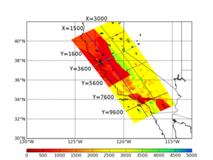
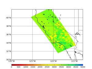
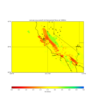
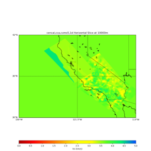
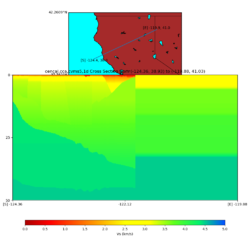
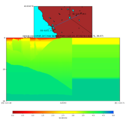
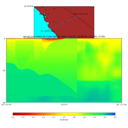
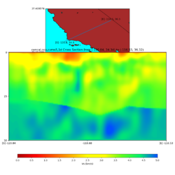
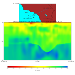
We have updated the CyberShake 18.5 velocity model to tile USGS Bay Area, CCA06, and CVM-S4.26. Also we have added the Ely GTL to the models. Then, we extracted horizontal cross-sections at 0 km, 0.1 km, 1 km, and 10 km. The 0 km cross-section also indicates the vertical cross-section locations.
Vs cross-sections
We have extracted horizontal cross-sections at 0 km, 0.1 km, 1 km, and 10 km. The 0 km cross-section also indicates the vertical cross-section locations.
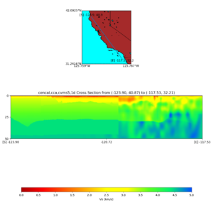
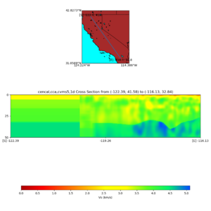
We extracted vertical cross-sections along 5 cuts parallel to the x-axis:
- Y index=1600: (38.929900, -124.363400) to (41.030000, -119.880200)
- Y index=3600: (37.413200, -123.140900) to (39.470700, -118.713500)
- Y index=5600: (35.884300, -121.967300) to (37.900400, -117.598200)
- Y index=7600: (34.344500, -120.838200) to (36.319900, -116.529600)
- Y index=9600: (32.794700, -119.750000) to (34.730300, -115.503600)
The southeast edge is on the left side of the plots.
and 2 cuts parallel to the y-axis:
- X index=1500: (40.866500, -123.900300) to (32.207800, -117.529700)
- X index=3000: (41.579900, -122.388500) to (32.844200, -116.127900)
The northwestern edge is on the left of the plots.
Verification
Performance Enhancements (over Study 17.3)
Computational and Data Estimates
Computational Estimates
In producing the computational estimates, we selected the four N/S/E/W extreme sites in the box which 1)within the 200 km cutoff for southern SAF events (381 sites) and 2)were outside the cutoff (488 sites). We produced inside and outside averages and scaled these by the number of inside and outside sites.
We also modified the box to be at an angle of 30 degrees counterclockwise of vertical, which makes the boxes about 15% smaller than with the previously used angle of 55 degrees.
We scaled our results based on the Study 17.3 performance of site s975, a site also in Study 18.3, and the Study 15.4 performance of DBCN, which used a very large volume and 100m spacing.
| # Grid points | #VMesh gen nodes | Mesh gen runtime | # GPUs | SGT job runtime | Titan SUs | BW node-hrs | |
|---|---|---|---|---|---|---|---|
| Inside cutoff, per site | 23.1 billion | 192 | 0.85 hrs | 800 | 1.35 hrs | 69.7k | 2240 |
| Outside cutoff, per site | 10.2 billion | 192 | 0.37 hrs | 800 | 0.60 hrs | 30.8k | 990 |
| Total | 41.6M | 1.34M |
For the post-processing, we quantified the amount of work by determining the number of individual rupture points to process (summing, over all ruptures, the number of rupture variations for that rupture times the number of rupture surface points) and multiplying that by the number of timesteps. We then scaled based on performance of s975 from Study 17.3, and DBCN in Study 15.4.
Below we list the estimates for Blue Waters or Titan.
| #Points to process | #Nodes (BW) | BW runtime | BW node-hrs | #Nodes (Titan) | Titan runtime | Titan SUs | |
|---|---|---|---|---|---|---|---|
| Inside cutoff, per site | 5.96 billion | 120 | 9.32 hrs | 1120 | 240 | 10.3 hrs | 74.2k |
| Outside cutoff, per site | 2.29 billion | 120 | 3.57 hrs | 430 | 240 | 3.95 hrs | 28.5k |
| Total | 635K | 42.2M |
One potential computational plan is to split the SGT calculations 25% BW/75% Titan, and split the PP the other way: 75% BW, 25% Titan. With a 20% margin, this would require 50.17M SUs on Titan, and 973K node-hrs on Blue Waters.
Currently we have 91.7M SUs available on Titan (expires 12/31/18), and 8.14M node-hrs on Blue Waters (expires 8/31/18). Based on the 2016 PRAC (spread out over 2 years), we budgeted approximately 6.2M node-hours for CyberShake on Blue Waters this year, of which we have used 0.01M.
Data Estimates
SGT size estimates are scaled based on the number of points to process.
| #Grid points | Velocity mesh | SGTs size | Temp data | Output data | |
|---|---|---|---|---|---|
| Inside cutoff, per site | 23.1 billion | 271 GB | 410 GB | 1090 GB | 19.1 GB |
| Outside cutoff, per site | 10.2 billion | 120 GB | 133 GB | 385 GB | 9.3 GB |
| Total | 158 TB | 216 TB | 589 TB | 11.6 TB |
If we plan on all the SGTs on Titan and split the PP 25% Titan, 75% Blue Waters, we will need:
Titan: 589 TB temp files + 3 TB output files = 592 TB
Blue Waters: 162 TB SGTs + 9 TB output files = 171 TB
SCEC storage: 1 TB workflow logs + 11.6 TB output data files = 12.6 TB(45 TB free)
Database usage: (4 rows PSA [@ 2, 3, 5, 10 sec] + 12 rows RotD [RotD100 and RotD50 @ 2, 3, 4, 5, 7.5, 10 sec])/rupture variation x 225K rupture variations/site x 869 sites = 3.1 billion rows x 125 bytes/row = 364 GB (2.0 TB free on moment.usc.edu disk)
Alternative Velocity Model Plots
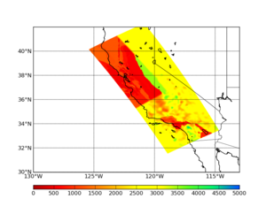
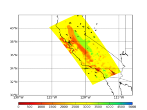
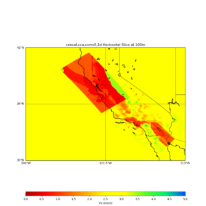
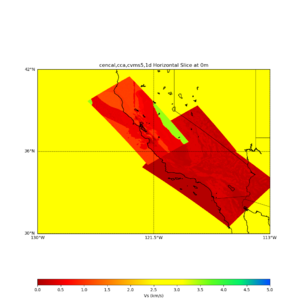
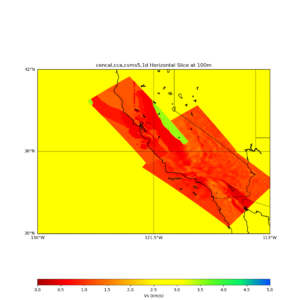
The following plots represent a proposed Northern California Velocity Model. Create using an updated version of the UCVM Software: The tiling order of velocity models in these plots is:
Science Name (ucvmc abbreviation):
- USGS Bay Area Model (cencal)
- CCA06 (cca)
- CVM-S4.26 (cvms5)
- Modified Hadley Kanamori 1D (1d)
Tiled without adding Ely-Jordan GTL to CCA06 or CVM-S4.26
Tiled with Ely-Jordan Vs30-based GTL added to CCA06, and CVM-S4.16
Tiled with Ely-Jordan Vs30-based GTL added to CCA06 and CVM-S4.26
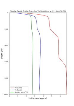
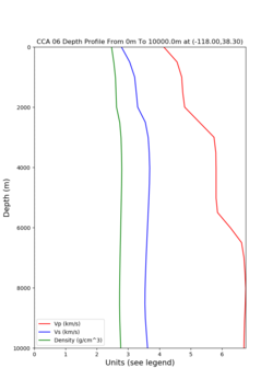
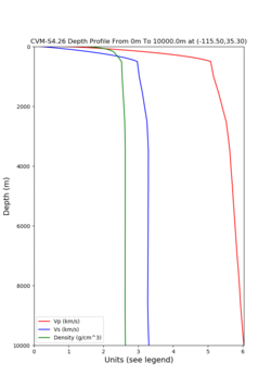
Depth profiles of 2 selected points:
- Point in CCA06 Model (38.3 -118.0 ):
- Point in CVM-S4.26 (35.3 -115.5) :
