Difference between revisions of "CyberShake Study 24.1"
| Line 327: | Line 327: | ||
! Y=2400 !! Y=4800 !! Y=7200 | ! Y=2400 !! Y=4800 !! Y=7200 | ||
|- | |- | ||
| − | | [[File: | + | | [[File:s3446_x_2400_smoothed_ss_bbp1d_vs.png|thumb|400px]] |
| − | | [[File: | + | | [[File:s3446_x_4800_smoothed_ss_bbp1d_vs.png|thumb|400px]] |
| − | | [[File: | + | | [[File:s3446_x_7200_smoothed_ss_bbp1d_vs.png|thumb|400px]] |
|} | |} | ||
| Line 335: | Line 335: | ||
! X=1400 !! X=2800 | ! X=1400 !! X=2800 | ||
|- | |- | ||
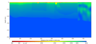
| − | | [[File: | + | | [[File:s3446_y_1400_smoothed_ss_bbp1d_vs.png|thumb|400px]] |
| − | | [[File: | + | | [[File:s3446_y_2800_smoothed_ss_bbp1d_vs.png|thumb|400px]] |
|} | |} | ||
Revision as of 21:09, 13 March 2024
CyberShake Study 24.1 is an upcoming study in Northern California which includes deterministic low-frequency (0-1 Hz) and stochastic high-frequency (1-50 Hz) simulations. We will use the Graves & Pitarka (2022) rupture generator and the high frequency modules from the SCEC Broadband Platform v22.4.
Contents
- 1 Status
- 2 Data Products
- 3 Science Goals
- 4 Technical Goals
- 5 Sites
- 6 Ruptures to Include
- 7 Velocity Model
- 8 Rupture Generator
- 9 High-frequency codes
- 10 Updates and Enhancements
- 11 Output Data Products
- 12 Computational and Data Estimates
- 13 Lessons Learned
- 14 Stress Test
- 15 Events During Study
- 16 Performance Metrics
- 17 Production Checklist
- 18 Presentations, Posters, and Papers
- 19 References
Status
This study is in the planning phase. We hope to begin this study in January 2024.
Data Products
Science Goals
The science goals for this study are:
- To perform an updated broadband study for the greater Bay Area.
- To use an updated rupture generator and improved velocity model from Study 18.8.
- To use the same parameters as in Study 22.12 when possible to make comparisons between the studies simple.
Technical Goals
The technical goals for this study are:
- Use Frontier for the SGTs and Frontera for the post-processing and high-frequency calculations.
- Use a modified approach for the production database, to improve performance.
Sites
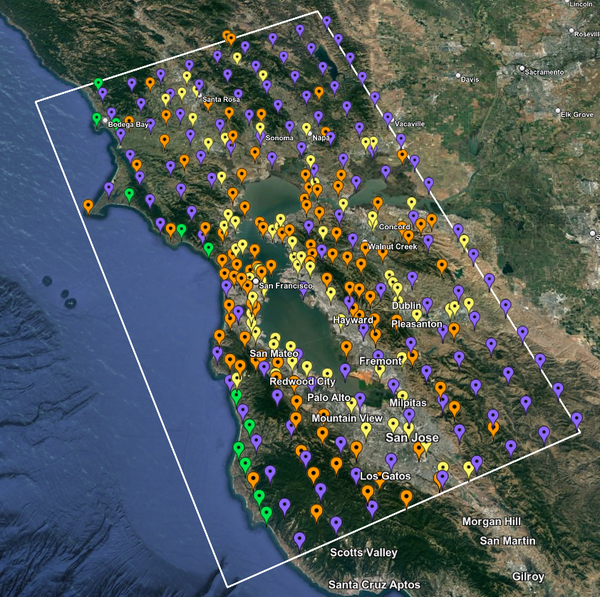
For this study, we chose to focus on a smaller region than in Study 18.8. Starting with the Study 18.8 region, we selected a smaller (180 km x 100 km) box extending roughly from San Jose to Santa Rosa, containing 315 sites.
|
Ruptures to Include
Summary: we decided to exclude the southern San Andreas events from Study 24.1. This was implemented by creating a new ERF with ID 64, which includes all the ERF 36 ruptures except for the southern San Andreas events.
Historically, we have determined which ruptures to include in a CyberShake run by calculating the distance between the site and the closest part of the rupture surface. If that distance is less than 200 km, we then include all ruptures which take place on that surface, including ruptures which may extend much farther away from the site than 200 km.
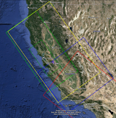
For Northern California sites, this means that sites around San Jose and south include southern San Andreas events (events which rupture the northernmost segment of the southern San Andreas) within 200 km. Since there are some UCERF2 ruptures which extend from the Parkfield segment all the way down to Bombay Beach, the simulation volumes for some of these Northern California sites cover most of the state. This was the case for Study 18.8 (sample volumes can be seen on this page). This required tiling together 3 3D models and a background 1D model.
To simplify the velocity model and reduce the volumes, we are investigating omitting southern San Andreas events from this study.
Source Contribution Curves
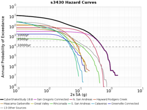
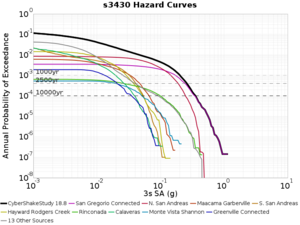
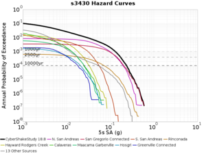
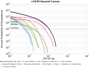
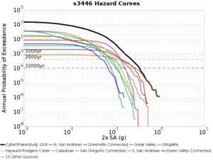
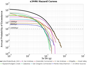
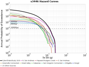
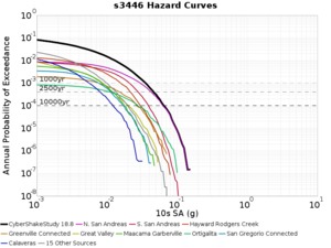
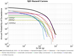
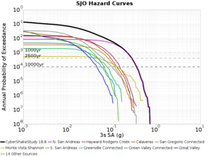
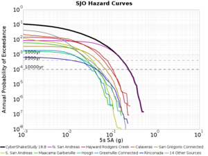
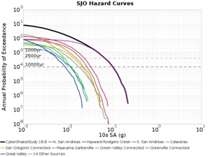
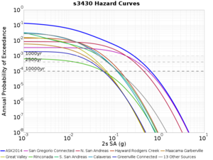
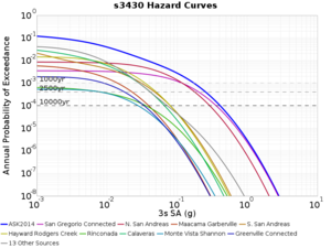
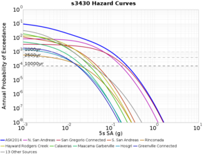
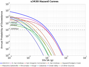
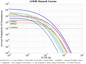
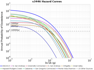
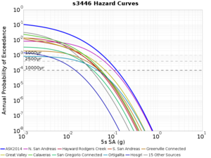
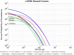
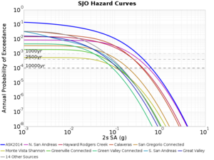
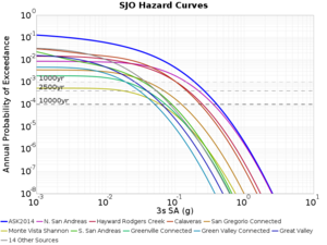
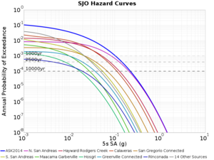
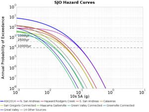
Below are source contribution curves for 3 sites: s3430 (southwest corner of the study region), s3446 (southeast corner of the study region), and SJO (San Jose). In general, the sSAF events are about the 3rd largest contributor at long periods and medium-to-long return periods.
| Site | 2 sec | 3 sec | 5 sec | 10 sec |
|---|---|---|---|---|
| s3430 | ||||
| s3446 | ||||
| SJO |
We also looked at the source contributions for these 3 sites from ASK 2014. In general, the sSAF events play a reduced role compared to the CyberShake results.
| Site | 2 sec | 3 sec | 5 sec | 10 sec |
|---|---|---|---|---|
| s3430 | ||||
| s3446 | ||||
| SJO |
Disaggregations
From Study 18.8, we looked at disaggregations for s3430, s3446, and SJO at 1e-3 (1000 yr), 4e-4 (2500 yr), and 1e-4 (10000 yr) probability levels, at 2 and 10 seconds. We list the top 3 contributing sources from the southern SAF, their magnitude ranges, and their contributing percentages.
The only significant contributions are for site s3446 at 10 second period. Those come from large events, with median magnitude 7.85 or higher.
s3430
| Period | 1e-3 | 4e-4 | 1e-4 |
|---|---|---|---|
| 2 sec | 80 (S. San Andreas;PK, M5.65-6.35), <0.01% 81 (S. San Andreas;PK+CH, M6.75-7.35), <0.01% 82 (S. San Andreas;PK+CH+CC, M7.15-7.65), <0.01% |
80 (S. San Andreas;PK, M5.65-6.35), <0.01% 81 (S. San Andreas;PK+CH, M6.75-7.35), <0.01% 82 (S. San Andreas;PK+CH+CC, M7.15-7.65), <0.01% |
80 (S. San Andreas;PK, M5.65-6.35), <0.01% 81 (S. San Andreas;PK+CH, M6.75-7.35), <0.01% 82 (S. San Andreas;PK+CH+CC, M7.15-7.65), <0.01% |
| 10 sec | 86 (S. San Andreas;PK+CH+CC+BB+NM+SM+NSB, M7.65-8.25), 0.01% 89 (S. San Andreas;PK+CH+CC+BB+NM+SM+NSB+SSB+BG+CO, M7.75-8.45), 0.01% 85 (S. San Andreas;PK+CH+CC+BB+NM+SM, M7.55-8.15), <0.01% |
89 (S. San Andreas;PK+CH+CC+BB+NM+SM+NSB+SSB+BG+CO, M7.75-8.45), <0.01% 80 (S. San Andreas;PK, M5.65-6.35), <0.01% 81 (S. San Andreas;PK+CH, M6.75-7.35), <0.01% |
80 (S. San Andreas;PK, M5.65-6.35), <0.01% 81 (S. San Andreas;PK+CH, M6.75-7.35), <0.01% 82 (S. San Andreas;PK+CH+CC, M7.15-7.65), <0.01% |
s3446
| Period | 1e-3 | 4e-4 | 1e-4 |
|---|---|---|---|
| 2 sec | 84 (S. San Andreas;PK+CH+CC+BB+NM, M7.45-7.95), <0.01% 89 (S. San Andreas;PK+CH+CC+BB+NM+SM+NSB+SSB+BG+CO, M7.75-8.45), <0.01% 80 (S. San Andreas;PK, M5.65-6.35), <0.01% |
80 (S. San Andreas;PK, M5.65-6.35), <0.01% 81 (S. San Andreas;PK+CH, M6.75-7.35), <0.01% 82 (S. San Andreas;PK+CH+CC, M7.15-7.65), <0.01% |
80 (S. San Andreas;PK, M5.65-6.35), <0.01% 81 (S. San Andreas;PK+CH, M6.75-7.35), <0.01% 82 (S. San Andreas;PK+CH+CC, M7.15-7.65), <0.01% |
| 10 sec | 85 (S. San Andreas;PK+CH+CC+BB+NM+SM, M7.55-8.15), 6.83% 86 (S. San Andreas;PK+CH+CC+BB+NM+SM+NSB, M7.65-8.25), 4.18% 84 (S. San Andreas;PK+CH+CC+BB+NM, M7.45-7.95), 1.53% |
85 (S. San Andreas;PK+CH+CC+BB+NM+SM, M7.55-8.15), 4.27% 86 (S. San Andreas;PK+CH+CC+BB+NM+SM+NSB, M7.65-8.25), 3.09% 89 (S. San Andreas;PK+CH+CC+BB+NM+SM+NSB+SSB+BG+CO, M7.75-8.45), 1.08% |
86 (S. San Andreas;PK+CH+CC+BB+NM+SM+NSB, M7.65-8.25), 1.19% 85 (S. San Andreas;PK+CH+CC+BB+NM+SM, M7.55-8.15), 1.19% 89 (S. San Andreas;PK+CH+CC+BB+NM+SM+NSB+SSB+BG+CO, M7.75-8.45), 0.55% |
SJO
| Period | 1e-3 | 4e-4 | 1e-4 |
|---|---|---|---|
| 2 sec | 80 (S. San Andreas;PK, M5.65-6.35), <0.01% 81 (S. San Andreas;PK+CH, M6.75-7.35), <0.01% 82 (S. San Andreas;PK+CH+CC, M7.15-7.65), <0.01% |
80 (S. San Andreas;PK, M5.65-6.35), <0.01% 81 (S. San Andreas;PK+CH, M6.75-7.35), <0.01% 82 (S. San Andreas;PK+CH+CC, M7.15-7.65), <0.01% |
80 (S. San Andreas;PK, M5.65-6.35), <0.01% 81 (S. San Andreas;PK+CH, M6.75-7.35), <0.01% 82 (S. San Andreas;PK+CH+CC, M7.15-7.65), <0.01% |
| 10 sec | 85 (S. San Andreas;PK+CH+CC+BB+NM+SM, M7.55-8.15), 0.09% 86 (S. San Andreas;PK+CH+CC+BB+NM+SM+NSB, M7.65-8.25), 0.07% 89 (S. San Andreas;PK+CH+CC+BB+NM+SM+NSB+SSB+BG+CO, M7.75-8.45), 0.05% |
89 (S. San Andreas;PK+CH+CC+BB+NM+SM+NSB+SSB+BG+CO, M7.75-8.45), 0.01% 88 (S. San Andreas;PK+CH+CC+BB+NM+SM+NSB+SSB+BG, M7.75-8.35), 0.01% 86 (S. San Andreas;PK+CH+CC+BB+NM+SM+NSB, M7.65-8.25), <0.01% |
80 (S. San Andreas;PK, M5.65-6.35), <0.01% 81 (S. San Andreas;PK+CH, M6.75-7.35), <0.01% 82 (S. San Andreas;PK+CH+CC, M7.15-7.65), <0.01% |
Velocity Model
We will perform validation of the proposed velocity model using northern California BBP events.
To line up closely with the USGS SF model angle, we will generate volumes using an angle of -36 degrees.
For generating sample meshes, we will use site s3446, a site in the SE corner of the study region with one of the larger volumes.
Primary 3D model
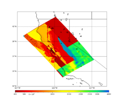
Given the extensive low-velocity near-surface regions in the USGS SF CVM, we plan to use a minimum Vs of 400 m/s (and therefore a grid spacing of 80 m).
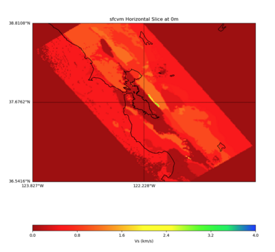
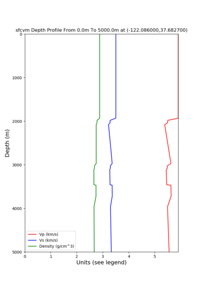
Initial slices with the USGS SF CVM are available here: UCVM_sfcvm_geomodelgrid. We found two sharply defined high-velocity patches visible on the surface slice, one in the East Bay near the mountains, and another near Gilroy. These are regions where the gabbro type goes to the surface, and so the SF CVM geological rules dictate that the high velocities go to the surface as well.
These patches are not present in the Vs30 models - for instance, for the point (37.6827, -122.086) SF CVM gives a surface Vs of about 3500 m/s, but Wills (2015) has Vs30=710 and Thompson (2018) has Vs30=702.
Potential modification to gabbro regions
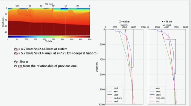
A candidate modification to the gabbro regions to reduce the near-surface velocities is to apply the approach used by Arben Pitarka and Rie Nakata, detailed below.
| Component | At surface | At 7.75 km depth | derivation |
|---|---|---|---|
| Vp | 4.2 km/s | 5.7 km/s | Linear interpolation |
| Vs | 2.44 km/s | 3.4 km/s | Vp/Vs relationship |
| Density | 2.76 g/cm3 | 2.87 g/cm3 | Vp/Density relationship |
The Vs (km/s) values are derived from Vp (km/s) using the San Leandro Gabbro relationship:
Vs = 0.7858 - 1.2344*Vp + 0.7949*Vp^2 - 0.1238*Vp^3 + 0.0064*Vp^4
The density (g/cm3) values are derived from Vp (km/s) using the San Leandro Gabbro relationship:
density = 2.4372 + 0.0761*Vp
A sample plot is below.
Background model
There are several candidates to use as a background model for the regions outside of the 3D model region.
1D models
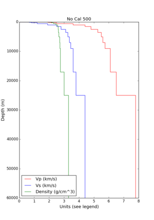
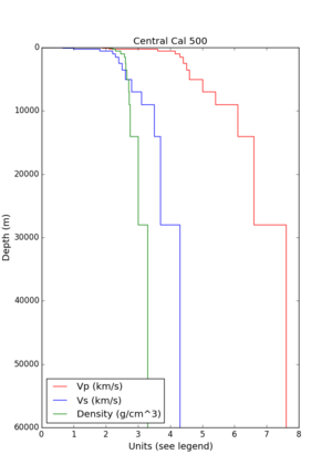
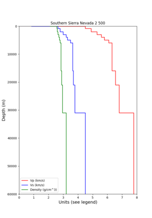
- 1D Broadband Platform model - either Northern California, Central California, or the Southern Sierras.
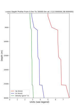
- 1D CVM-S4 background model
- Extend eastern edge of SFCVM model to fill the remaining volume
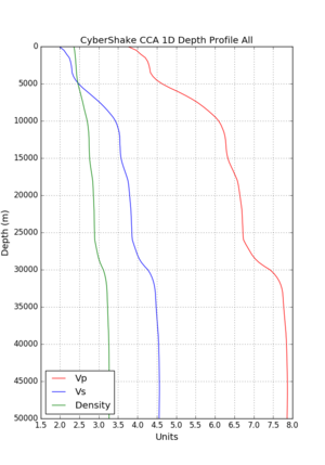
- 1D CCA model (derived from averaging CCA-06), used in Study 17.3
3D models
- 3D CANVAS long-period tomography model
- 3D National Crustal model
Plots of these options are available below.
| 1D Model | BBP NorCal | BBP CenCal | BBP SouthernSierras | CVM-S4.26.M01 1D background | CCA 1D |
|---|---|---|---|---|---|
| Plot |
Cross-sections
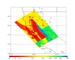
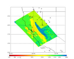
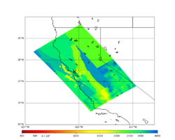
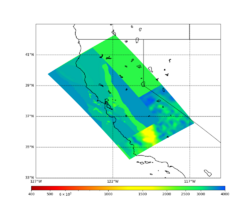
Cross-sections, no smoothing, CVM-S4.26.M01 1D background
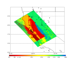
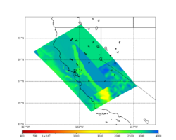
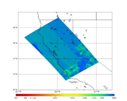
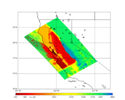
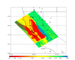
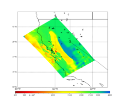
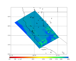
Below are horizontal cross-sections at various depths taken from a model for s3446 generated without smoothing, with the tiling SFCVM, CCA-06, CVM-S4.26.M01. This model was extracted on 2/28/24, and is one of the largest volumes needed for the study.
| 0m | 80m | 800m | 2000m | 4000m | 10000m |
|---|---|---|---|---|---|
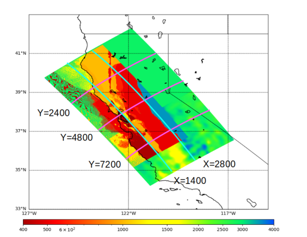
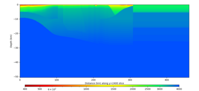
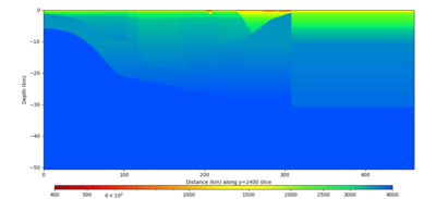
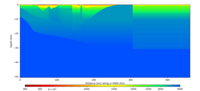
Below are vertical cross-sections taken from a model for s3446 generated without smoothing, with the tiling SFCVM, CCA-06, CVM-S4.26.M01. This model was extracted on 2/28/24, and is one of the largest volumes needed for the study.
| Y=2400 | Y=4800 | Y=7200 |
|---|---|---|
| X=1400 | X=2800 |
|---|---|
Cross-sections, smoothing, CVM-S4.26.M01 1D background
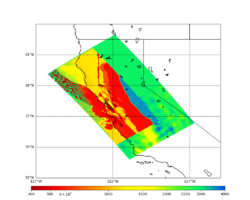
Below are horizontal cross-sections at various depths taken from a model for s3446 generated with smoothing, with the tiling SFCVM, CCA-06, CVM-S4.26.M01. This model was extracted on 2/28/24.
| 0m | 80m | 800m | 2000m | 4000m | 10000m |
|---|---|---|---|---|---|
Below are vertical cross-sections taken from a model for s3446 generated with smoothing, with the tiling SFCVM, CCA-06, CVM-S4.26.M01. This model was extracted on 2/28/24.
| Y=2400 | Y=4800 | Y=7200 |
|---|---|---|
| X=1400 | X=2800 |
|---|---|
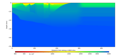
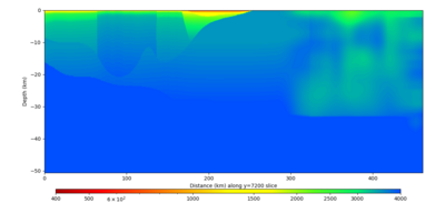
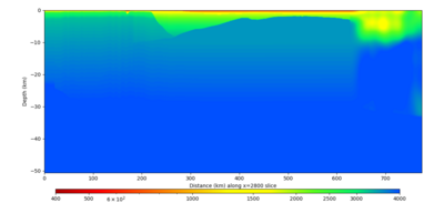
Cross-sections, no smoothing, Southern Sierra BBP 1D background
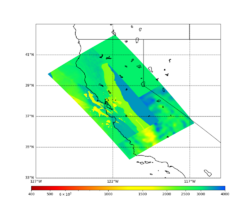
Below are horizontal cross-sections at various depths taken from a model for s3446 generated without smoothing, with the tiling SFCVM, CCA-06, Southern Sierra BBP1D model. This model was extracted on 3/13/24.
| 0m | 80m | 800m | 2000m | 4000m | 10000m |
|---|---|---|---|---|---|
Below are horizontal cross-sections at various depths taken from a model for s3446 generated without smoothing, with the tiling SFCVM, CCA-06, Southern Sierra BBP1D model. This model was extracted on 3/13/24.
| Y=2400 | Y=4800 | Y=7200 |
|---|---|---|
| X=1400 | X=2800 |
|---|---|
Rupture Generator
We will use the same version of the rupture generator that we used for Study 22.12, v5.5.2.
High-frequency codes
We will use the Graves & Pitarka high-frequency codes from the BBP v22.4.
However, since we are using a denser mesh (80m) and a lower minimum Vs (400 m/s), we will not apply site correction to the low-frequency seismograms before combining. Rob states, You may recall that there is a klugy process we have used to estimate the Vref value based on the Vsmin and grid spacing of the model. But, it has only been applied for the case of h=100 m and Vsmin=500 m/s. What I found here is that estimating Vref using the 80m & 400m/s model is that Vref is almost always less than Vs30 (i.e., Vsite). This means that when the site adjustment is applied, the motions are deamplified. This is why we see such a poor fit for the 3D case when using the estimated Vref values. My conclusion at this point is that if we run the 3D calculation with 80 m grid spacing and Vsmin of 400 m/s (or lower), then we probably do not need to apply any site adjustments.
Updates and Enhancements
- Used smaller study region than in Study 18.8.
- Removed southern San Andreas events, and created a new ERF.
Output Data Products
File-based data products
We plan to produce the following data products, which will be stored at CARC:
Deterministic
- Seismograms: 2-component seismograms, 8000 timesteps (400 sec) each.
- PSA: We are removing geometric mean PSA calculations from this study.
- RotD: PGV, and RotD50, the RotD50 azimuth, and RotD100 at 27 periods (20, 17, 15, 13, 12, 10, 8.5, 7.5, 6.5, 6, 5.5, 5, 4.4, 4, 3.5, 3, 2.8, 2.6, 2.4, 2.2, 2, 1.7, 1.5, 1.3, 1.2, 1.1, 1)
- Fourier spectra at 27 periods (20, 17, 15, 13, 12, 10, 8.5, 7.5, 6.5, 6, 5.5, 5, 4.4, 4, 3.5, 3, 2.8, 2.6, 2.4, 2.2, 2, 1.7, 1.5, 1.3, 1.2, 1.1, 1)
- Durations: for X and Y components, energy integral, Arias intensity, cumulative absolute velocity (CAV), and for both velocity and acceleration, 5-75%, 5-95%, and 20-80%. Also, period-dependent acceleration 5-75%, 5-95%, and 20-80% for 27 periods (20, 17, 15, 13, 12, 10, 8.5, 7.5, 6.5, 6, 5.5, 5, 4.4, 4, 3.5, 3, 2.8, 2.6, 2.4, 2.2, 2, 1.7, 1.5, 1.3, 1.2, 1.1, 1).
Broadband
- Seismograms: 2-component seismograms, 40000 timesteps (400 sec) each.
- PSA: We are removing geometric mean PSA calculations from this study.
- RotD: PGA, PGV, and RotD50, the RotD50 azimuth, and RotD100 at 68 periods (20, 17, 15, 13, 12, 10, 8.5, 7.5, 6.5, 6, 5.5, 5, 4.4, 4, 3.5, 3, 2.8, 2.6, 2.4, 2.2, 2, 1.7, 1.5, 1.3, 1.2, 1.1, 1, 0.85, 0.75, 0.65, 0.6, 0.55, 0.5, 0.45, 0.4, 0.35, 0.3, 0.28, 0.26, 0.24, 0.22, 0.2, 0.17, 0.15, 0.13, 0.12, 0.11, 0.1, 0.085, 0.075, 0.065, 0.06, 0.055, 0.05, 0.045, 0.04, 0.035, 0.032, 0.029, 0.025, 0.022, 0.02, 0.017, 0.015, 0.013, 0.012, 0.011, 0.01)
- Fourier spectra at 68 periods (20, 17, 15, 13, 12, 10, 8.5, 7.5, 6.5, 6, 5.5, 5, 4.4, 4, 3.5, 3, 2.8, 2.6, 2.4, 2.2, 2, 1.7, 1.5, 1.3, 1.2, 1.1, 1, 0.85, 0.75, 0.65, 0.6, 0.55, 0.5, 0.45, 0.4, 0.35, 0.3, 0.28, 0.26, 0.24, 0.22, 0.2, 0.17, 0.15, 0.13, 0.12, 0.11, 0.1, 0.085, 0.075, 0.065, 0.06, 0.055, 0.05, 0.045, 0.04, 0.035, 0.032, 0.029, 0.025, 0.022, 0.02, 0.017, 0.015, 0.013, 0.012, 0.011, 0.01)
- Durations: for X and Y components, energy integral, Arias intensity, cumulative absolute velocity (CAV), and for both velocity and acceleration, 5-75%, 5-95%, and 20-80%. Also, period-dependent acceleration 5-75%, 5-95%, and 20-80% for 68 periods (20, 17, 15, 13, 12, 10, 8.5, 7.5, 6.5, 6, 5.5, 5, 4.4, 4, 3.5, 3, 2.8, 2.6, 2.4, 2.2, 2, 1.7, 1.5, 1.3, 1.2, 1.1, 1, 0.85, 0.75, 0.65, 0.6, 0.55, 0.5, 0.45, 0.4, 0.35, 0.3, 0.28, 0.26, 0.24, 0.22, 0.2, 0.17, 0.15, 0.13, 0.12, 0.11, 0.1, 0.085, 0.075, 0.065, 0.06, 0.055, 0.05, 0.045, 0.04, 0.035, 0.032, 0.029, 0.025, 0.022, 0.02, 0.017, 0.015, 0.013, 0.012, 0.011, 0.01)
Database data products
We plan to store the following data products in the database on moment-carc:
Deterministic
- RotD50 for 6 periods (10, 7.5, 5, 4, 3, 2). Note that we are NOT storing RotD100.
- Duration: acceleration 5-75% and 5-95%, for both X and Y, and acceleration 5-75% and 5-95% for 6 periods (10, 7.5, 5, 4, 3, 2).
Broadband
- RotD50 for PGA, PGV, and 19 periods (10, 7.5, 5, 4, 3, 2, 1, 0.75, 0.5, 0.4, 0.3, 0.2, 0.1, 0.075, 0.05, 0.04, 0.03, 0.02, 0.01). Note that we are NOT storing RotD100.
- Duration: acceleration 5-75% and 5-95%, for both X and Y, and acceleration 5-75% and 5-95% for 19 periods (10, 7.5, 5, 4, 3, 2, 1, 0.75, 0.5, 0.4, 0.3, 0.2, 0.1, 0.075, 0.05, 0.04, 0.03, 0.02, 0.01).
Hazard products
For each site, we will produce hazard curves from the deterministic results at 10, 5, 3, and 2 seconds, and from the broadband results at 10, 5, 3, 2, 1, 0.5, 0.2, and 0.1 seconds.
When the study is complete, we will produce maps from the deterministic results at 10, 5, 3, and 2 seconds, and from the broadband results at 10, 5, 3, 2, 1, 0.5, 0.2, and 0.1 seconds.
