CyberShake MareNostrum Training

This page provides training for running the CyberShake TEST site on MareNostrum (MN4)

Videos

Recordings from the live training sessions are available below:

February 2, 2020 (1:04, 157 MB). Covers the overview, database, and jobs involved in SGT creation.

April 22, 2020 (1:12, 405 MB). Covers the post-processing jobs, data products jobs, and how to extend CyberShake to include new models.

Training overview

The goal of this training is to get you to run by hand all the steps involved in a CyberShake run. Here are the basic steps involved in the training:

Set up needed files
Initialize database with run information
Create Strain Green Tensors
Create synthetic seismograms and intensity measures
Create final data products

Actions you need to take will be in bold.

Terminal commands and output will be in this font.
My username is pr1ejg10 and my project is pr1ejg00.  Replace <username> or <working dir> with your username or your working directory, respectively.

Set up needed files

Create a directory to work from. I recommend something in scratch.

pr1ejg10@login2:~> cd /gpfs/scratch/pr1ejg00/<username>
pr1ejg10@login2:/gpfs/scratch/pr1ejg00/pr1ejg10> mkdir TEST
pr1ejg10@login2:/gpfs/scratch/pr1ejg00/pr1ejg10> cd TEST

An overview of the code involved in CyberShake is provided here. For this test, we are using the SGT-related codes, the PP-related codes, and the Data Products codes, but not the Stochastic codes.

Since MN4 does not permit outgoing connections, it is impossible to install CyberShake on MN4 directly from the repository. For the purposes of this training, I suggest you use my install directly. My CyberShake installation is located at:

/gpfs/projects/pr1ejg00/CyberShake

Due to the outgoing connection problem, on MN4 we are using a local SQLite database rather than a remote MySQL database, which is what SCEC's CyberShake install uses. Each trainee should work from their own database.

Copy in my training database from /gpfs/projects/pr1ejg00/CyberShake/database/training.sqlite.

pr1ejg10@login2:/gpfs/scratch/pr1ejg00/pr1ejg10/TEST> cp /gpfs/projects/pr1ejg00/CyberShake/database/training.sqlite .

In order to look at this database, we need sqlite. Add the SQLite module to your environment.

pr1ejg10@login2:/gpfs/scratch/pr1ejg00/pr1ejg10/TEST> module load sqlite

Let's examine this database. Use sqlite3 to investigate the tables.

pr1ejg10@login2:/gpfs/scratch/pr1ejg00/pr1ejg10/TEST> sqlite3 training.sqlite
SQLite version 3.20.0 2017-07-10 19:08:59
Enter ".help" for usage hints.
sqlite> .tables
CyberShake_Runs                      IM_Types                           
CyberShake_Site_Regions              PeakAmplitudes                     
CyberShake_Site_Ruptures             Rupture_Variation_Scenario_IDs     
CyberShake_Site_Types                Rupture_Variation_Scenario_Metadata
CyberShake_Sites                     Rupture_Variations                 
ERF_IDs                              Ruptures                           
ERF_Metadata                         SGT_Variation_IDs                  
ERF_Probability_Models               Studies                            
Hazard_Curve_Points                  Velocity_Model_Metadata            
Hazard_Curves                        Velocity_Models                    
Hazard_Datasets     
sqlite> .schema Velocity_Models
CREATE TABLE Velocity_Models
(
Velocity_Model_ID integer primary key AUTOINCREMENT not null ,
Velocity_Model_Name varchar(50) not null,
Velocity_Model_Version varchar(50) not null
);
sqlite> select * from Velocity_Models;
1|CVM-S4.26|4.26

I have pre-inserted some of the setup you'll need, such as Ruptures, Rupture_Variations, and CyberShake_Site_Ruptures. For queries and insertions, SQLite uses practically identical syntax to MySQL. To quit, type .quit.

Note that not all the tables defined in the full CyberShake schema are in this test database.

Initialize database with run information

CyberShake keeps track of what we call 'runs' in the database. A run is a full CyberShake calculation for a single site.

When we run large CyberShake studies, we have scripts which automatically create runs as part of our workflows. For this test, we will populate the database ourselves.

Create a database entry for our test run.

sqlite> select * from CyberShake_Sites;
1|CyberShake Verification Test - USC|TEST|34.0192|-118.286|1
sqlite> select * from Velocity_Models;
1|CVM-S4.26|4.26
sqlite> select * from ERF_IDs;
35|WGCEP (2007) UCERF2 - Single Branch|Mean UCERF 2 - Single Branch Earthquake Rupture Forecast FINAL|1|1
36|WGCEP (2007) UCERF2 - Single Branch 200m| Mean UCERF 2 - Single Branch Earthquake Rupture Forecast FINAL, 200m|1|1
sqlite> select * from SGT_Variation_IDs;
1|AWP_ODC_SGT|SGTs generated with AWP-ODC-SGT with Qp=Qs=10000
2|AWP_ODC_SGT GPU|SGTs generated with AWP-ODC-SGT GPU
sqlite> select * from Rupture_Variation_Scenario_IDs;
1|36|genslip-v3.3.1b|Graves & Pitarka (2014) with uniform grid down dip hypocenter location, modified rupture variation constant
insert into CyberShake_Runs(Site_ID, ERF_ID, SGT_Variation_ID, Velocity_Model_ID, Rup_Var_Scenario_ID, Status, Status_Time, Last_User, Max_Frequency, Low_Frequency_Cutoff, SGT_Source_Filter_Frequency) values (1, 36, 1, 1, 1, "SGT Started", "2020-02-14 12:00:00", "<username>", 0.5, 0.5, 1.0);

Determine the run ID, which you'll use for your test.

sqlite> select Run_ID from CyberShake_Runs;
1

Exit sqlite. We're done with it for now.

sqlite> .quit

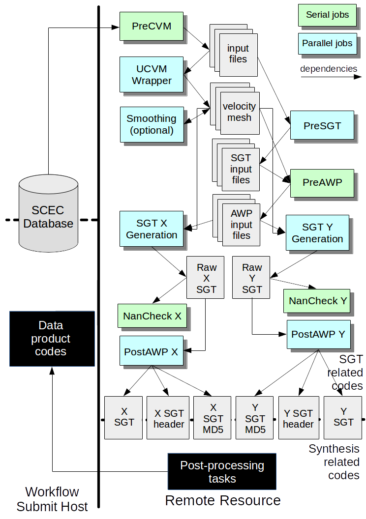
Create Strain Green Tensors

As outlined here, there are 7 jobs we need to run to generate SGTs for our test site.

PreCVM

Details about this stage are available here. This stage may be modified for Iceland, since each site may end up using the same volume. Note that the volume dimensions must be evenly divisible by the number of cores in that dimension.

Copy over my PreCVM batch script from /gpfs/scratch/pr1ejg00/pr1ejg10/TEST/precvm.slrm .

pr1ejg10@login2:/gpfs/scratch/pr1ejg00/pr1ejg10/TEST> cp /gpfs/scratch/pr1ejg00/pr1ejg10/TEST/precvm.slrm .

Edit the batch script. Change the sqlite path (--server sqlite:...) to point to your sqlite file instead of mine.
Submit the job, using sbatch. When complete, make sure there are no errors in precvm.e .

UCVM

PreCVM must finish before you can run this stage.

Details about this stage are available here. This stage will not be part of the Icelandic processing - you won't use UCVM to create a velocity model - but some other code will provide one.

Copy over my UCVM batch script from /gpfs/scratch/pr1ejg00/pr1ejg10/TEST/ucvm.slrm .
Submit the job. When complete, make sure there are no errors in ucvm.e .This is a parallel job, and may wait in the queue for some time before running.

PreSGT

PreCVM must finish before you can run this stage, but it can run concurrently with UCVM.

Details about this stage are available here.

Copy over my PreSGT batch script from /gpfs/scratch/pr1ejg00/pr1ejg10/TEST/presgt.slrm .
Submit the job. When complete, make sure there are no errors in presgt.e .

PreAWP

UCVM and PreSGT must finish before you can run this stage. Note that we're skipping the Smoothing step, since we're only using a single velocity model.

Details about this stage are available here.

Copy over my PreAWP batch script from /gpfs/scratch/pr1ejg00/pr1ejg10/TEST/preawp.slrm .
Edit the script. Change '--run-id 1' to use your correct run id, which might not be 1.
Submit the job. When complete, make sure there are no errors in preawp.e .

SGT

PreAWP must finish before you can run this stage.

Details about this stage are available here.

We run two SGTs, one for each horizontal component. They can run concurrently. PreAWP set up the input files needed for both horizontal components. If you'd like to run the vertical also, you'd need to make changes to PreAWP.

Copy over my SGT x and SGT y batch scripts from /gpfs/scratch/pr1ejg00/pr1ejg10/TEST/awp_x.slrm and awp_y.slrm .
Submit the job. When complete, check awp_x.e and awp_y.e .

Note: The following floating-point exceptions are signalling: IEEE_INVALID_FLAG IEEE_UNDERFLOW_FLAG IEEE_DENORMAL

This is OK and is not an error.

This job runs on 1700 cores, so you may need to wait in the queue for a while before it runs.

NaNCheck

We run two of these as well, one for each horizontal component. The SGT for that component must finish before you can run this stage.

Details about this stage are available here.

Copy over my check batch scripts from /gpfs/scratch/pr1ejg00/pr1ejg10/TEST/check_x.slrm and check_y.slrm .
Submit the jobs. When complete, make sure there are no errors in check_x.e or check_y.e .

PostAWP

We also run two of these. The SGT for the component must finish before you can run this stage, but it can run concurrently with NaNCheck.

Details about this stage are available here.

Copy over my post batch scripts from /gpfs/scratch/pr1ejg00/pr1ejg10/TEST/post_x.slrm and post_y.slrm .
Change the RUN_ID variable to be set to your run ID.
Submit the jobs. When complete, make sure there are no errors in post_x.e or post_y.e .

Congratulations, you have generated a pair of SGTs!

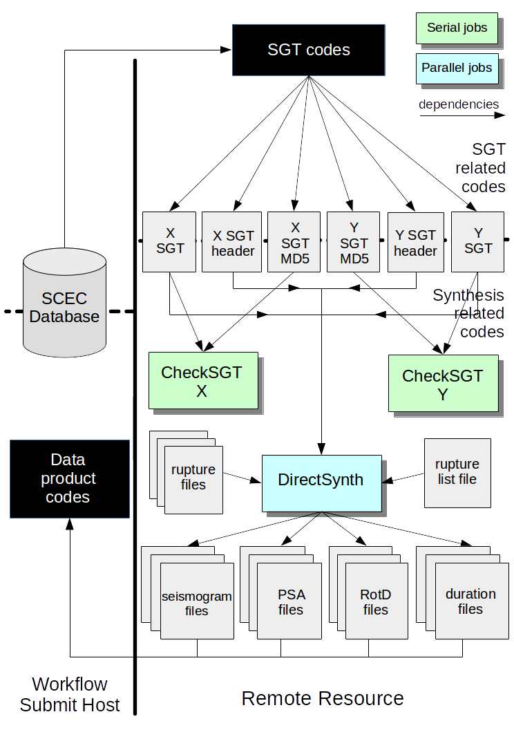
Post-processing

The post-processing steps are illustrated in this diagram. Since you're not moving the SGTs between systems, we can skip the md5sum check stage, so we only have one stage to run.

Details about DirectSynth, the seismogram synthesis stage, are available here .

This step requires a bit more setup than the previous ones. We must provide a list of all the ruptures which need their seismograms synthesized, and typically I symlink both the rupture geometry files (from which rupture variations are generated), the SGT files, and their headers.

Create a directory for the post-processing inside your working directory.

pr1ejg10@login2:/gpfs/scratch/pr1ejg00/pr1ejg10/TEST> mkdir post-processing
pr1ejg10@login2:/gpfs/scratch/pr1ejg00/pr1ejg10/TEST> cd post-processing

Copy in the rupture file list from /gpfs/scratch/pr1ejg00/pr1ejg10/TEST/post-processing/rupture_file_list_TEST .
Symlink the *.sgt and *.sgthead files you created earlier into the post-processing directory.

pr1ejg10@login2:/gpfs/scratch/pr1ejg00/pr1ejg10/TEST/post-processing> ln -s ../TEST_fx_<run id>.sgt
pr1ejg10@login2:/gpfs/scratch/pr1ejg00/pr1ejg10/TEST/post-processing> ln -s ../TEST_fx_<run id>.sgthead
pr1ejg10@login2:/gpfs/scratch/pr1ejg00/pr1ejg10/TEST/post-processing> ln -s ../TEST_fy_<run id>.sgt
pr1ejg10@login2:/gpfs/scratch/pr1ejg00/pr1ejg10/TEST/post-processing> ln -s ../TEST_fy_<run id>.sgthead

Create symlinks to all the rupture geometry files. You can use my helper script, /gpfs/scratch/pr1ejg00/pr1ejg10/TEST/post-processing/make_lns.py.

pr1ejg10@login2:/gpfs/scratch/pr1ejg00/pr1ejg10/TEST/post-processing> /gpfs/scratch/pr1ejg00/pr1ejg10/TEST/post-processing/make_lns.py rupture_file_list_TEST /gpfs/projects/pr1ejg00/CyberShake/ruptures/Ruptures_erf36

Copy in the batch script from /gpfs/scratch/pr1ejg00/pr1ejg10/TEST/post-processing/run_ds.slrm .
Edit run_ds.slrm so RUN_ID uses the correct run id.
Run the job. This one may also take a while in the queue.
Check two places for errors. Check both the end of ds.e, and also the end of log.84. At the end of log.84 you should see something like:

Jan 24 20:55:45.870309> Sending complete message to process 83.
Jan 24 20:55:45.870318> Sending message to processor 83.
Jan 24 20:55:45.870326> Shutting down.

When complete, you will have 395 Seismogram, PeakVals, RotD, and Duration files. File formats are described in detail here.

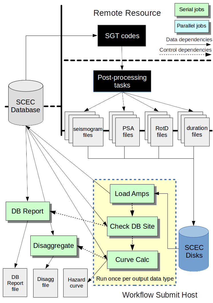
Data Product generation

Once the seismograms and IM files are generated, the IMs can be put into the database and a variety of data products generated. The jobs involved in the typical CyberShake workflow are illustrated in this diagram.

For this test, we aren't going to run all the jobs, just the Load Amps, the Check, and the Curve Calc for the RotD files.

Load Amps

Details about this stage are available here.

We will point to the SQLite database for database population. I've created a helper script for this purpose.

Change directories back to your top-level working directory, not the post-processing one.

pr1ejg10@login2:/gpfs/scratch/pr1ejg00/pr1ejg10/TEST/post-processing> cd ..

Copy over my helper script from /gpfs/scratch/pr1ejg00/pr1ejg10/TEST/db_insert.sh .
Edit the script. Change '-server sqlite:...' to point to your training.sqlite file that you used earlier in the training.
Run the script. It will print output as it goes.

Check DB

Details about this stage are available here. Basically, this task verifies that all the IMs were correctly inserted into the database.

Copy over my helper script from /gpfs/scratch/pr1ejg00/pr1ejg10/TEST/check_db.sh .
Edit the script. You'll need to change both the sqlite file it points to, and also the run id (the -r argument).
Run the script. It will print output as it goes. Check for errors.

Curve Calc

Details about this stage are available here .

Before we can calculate curves, we need to have a corresponding Hazard_Dataset in the database. This only needs to be done once for a given combination of velocity model, SGT variation, rupture scenario, and ERF.

Create an appropriate Hazard Dataset. First, get the IDs you'll need from your CyberShake_Runs table, then use it to populate Hazard Datasets.

sqlite> select ERF_ID, Rup_Var_Scenario_ID, SGT_Variation_ID, Velocity_Model_ID from CyberShake_Runs where Run_ID=<run id>;
36|1|1|1
sqlite> insert into Hazard_Datasets (ERF_ID, Rup_Var_Scenario_ID, SGT_Variation_ID, Velocity_Model_ID, Prob_Model_ID, Time_Span_ID, Max_Frequency, Low_Frequency_Cutoff) values (36, 1, 1, 1, 1, 1, 0.5, 0.5)

Copy over my helper script from /gpfs/scratch/pr1ejg00/pr1ejg10/TEST/curve_calc.sh .
Edit the script. Replace the first argument, the path to the sqlite file (/gpfs/projects/pr1ejg00/CyberShake/database/test.sqlite in mine) with the path to your database. Also, replace the --run-id with the correct one for your test.
Run the script. It will print output as it goes.

Congratulations! You have calculated CyberShake hazard curves! You can access them either by looking at the *.pdf and *.png files you've created, or by using sqlite to examine the values in the database directly.

Verification

To confirm that you got the right answers, compare one of your hazard curves with the one I generated.

Use sqlite to load your database.

Run a query to get your 3 sec RotD50 curve.

sqlite> select P.X_Value, P.Y_Value from Hazard_Curve_Points P, Hazard_Curves C where C.Run_ID=1 and C.Hazard_Curve_ID=P.Hazard_Curve_ID and C.IM_Type_ID=162;

Compare your curve to mine. Ideally the values will match exactly, but in general anything with differences of O(0.01%) is fine. For the 3 second RotD50 curve, the reference values (the values I got when I ran the code) are:

X value	Y value
0.005	0.00669446347113578
0.007	0.00669446347113578
0.0098	0.00668048983780867
0.0137	0.00665296801989335
0.0192	0.00651297322733557
0.0269	0.00630546899968387
0.0376	0.00576024330858993
0.0527	0.00509651492213958
0.0738	0.00416060395812046
0.103	0.00279691975696716
0.145	0.00166295938324768
0.203	0.000834190556129544
0.284	0.000362477682089857
0.397	0.0001266222803048
0.556	2.71102060581674e-05
0.778	4.75466199389984e-06
1.09	1.86439212512823e-07
1.52	0.0
2.13	0.0

Extending CyberShake

Once you have the basic CyberShake install configured, you can augment it with additional data for a new model or region. Below are details about what needs to be done to include new data.

Earthquake Rupture Forecast

Adding a new earthquake rupture forecast require several different modifications.

Ruptures

First, you should add information for the new ruptures (the fault surfaces). This consists of both database additions and the creation of rupture geometry files.

Add new entries to the database.
1. Create a new ERF in the ERF_IDs table. Provide a name, description, and default probability model (cross-referenced with the ERF_Probability_Models table) and default time span (cross-referenced with the Time_Spans table).
2. Optionally, add metadata to the ERF_Metadata table. This can be used to track certain ERF parameters you might want to access individually.
3. Populate the Ruptures table. In California CyberShake, we use the UCERF2 conventions for source and rupture. A source is a named fault section, usually with a consistent fault geometry, and a rupture has an assigned probability and magnitude. For each entry in the table, you will need to specify the following:
  - Identifying information: source id, rupture id, name. The source id and rupture id are how CyberShake tracks individual ruptures, so the (source id, rupture id) tuples must be unique.
  - Magnitude
  - Probability. Probabilities of individual events are calculated by dividing the rupture probability by the number of variations for the rupture.
  - Information about the rupture geometry. In CyberShake, rupture surfaces are represented by a grid of points. The seismograms are simulated by calculating the contribution from each point as a point source and then combined. Specifically, the database tracks grid spacing (spacing between rupture surface points), number of rows, number of columns, and total points.
  - The geographic extent of the rupture is needed so CyberShake can calculate how large the simulation volume must be. Thus, the database stores the 3D coordinates of opposite corners of the rupture surface. It doesn't matter which pair of opposite corners is used, or in what order.
Create rupture geometry files, one per rupture. These files should follow the format specified here. The values in the headers of these files should match the values found in the database. I recommend using the UCERF2 approach for rectangular rupture surfaces, and the RSQSim one for triangular or irregular meshes.
Stage the rupture geometry files. The root directory for rupture files is specified as RUPTURE_ROOT in the cybershake.cfg file, in <CyberShake root dir>/software/cybershake.cfg. CyberShake assumes that the rupture files for ERF X are stored in ${RUPTURE_ROOT}/Ruptures_erf<X>/<source id>/<rupture id>/<source id>_<rupture id>.txt , so you will want to copy your rupture geometry files there.

Rupture Variations

CyberShake supports two modes of synthesizing rupture variations:

Rupture geometries, but no explicit slip time histories, are provided. The rupture geometries are passed through a Graves & Pitarka rupture generator, which is integrated with the DirectSynth code, to generate individual realizations, which are then used to perform the seismogram syntheis.
Both rupture geometries and slip time histories are provided. The rupture generator is bypassed, and each individual slip time history is used to produce a seismogram.

From our conversations, I believe the plan is to use approach #1, so I will outline the steps involved there in setting up the database.

If using a new GP generator, create a rupture variation scenario entry in the Rupture_Variation_Scenario_IDs table. This is used to track what version and parameters of the GP rupture generator code are used, since the same ERF could be used with multiple rupture variations. You will need to specify a name and a description.
If using a new GP generator, add any necessary metadata to the Rupture_Variation_Scenario_Metadata. This is useful for verification and reproducibility.
Add new entries to the Rupture_Variations table. This table is used by CyberShake to determine which rupture variations go with a given ERF, rupture variation scenario, source, and rupture. Every rupture variation for a given ERF and scenario will have a unique (source id, rupture id, rupture variation id) tuple. You should also include the Rup_Var_LFN, which stands for 'Logical File Name', and should be something unique -- for example, 'e36_rv6_128_1.txt.variation-r000000' for ERF 36, rupture variation scenario id 6, source 128, rupture 1, rupture variation 0. Including the hypocenter locations is optional.

Sites

Adding new sites is straightforward.

Create a new entry in the CyberShake_Sites table for each site. You'll need to specify the site name, a 5-character or less short name, the latitude and longitude, and an optional site type, which cross-references with the CyberShake_Site_Types table.
Populate the CyberShake_Site_Ruptures table. This table is used to determine which ruptures should be simulated for a given site. CyberShake internally applies no cutoffs, so any ruptures included in this table will be simulated. For each site, you should add a row for each rupture that should be included when running CyberShake simulations for that site.
The CyberShake_Site_Regions table is no longer used -- regions are dynamically calculated from the rupture geometries -- so it doesn't need to be populated.

Velocity Models

There are two main approaches to adding new velocity models.

Register a new model into UCVM. This requires multiple manual steps, and should be done in coordination with the SCEC software group.
Create a new execution stage which can replace UCVM. For a simple model, this is easier than integrating it into UCVM. Some things to keep in mind:
- The generated mesh should be in AWP format to interface with the SGT code.
- If only one model is being used, the smoothing stage can be skipped.
- If not guaranteed, the mesh should be post-processed to verify that all Vs values are above the minimum (and if adjustments are necessary, that Vp and rho are scaled).
- For all points in the mesh, Vp/Vs >= 1.45 for numerical convergence.

With either approach, be sure to add the new velocity model into the Velocity_Models table.

CyberShake MareNostrum Training

Contents

Videos

Training overview

Set up needed files

Initialize database with run information

Create Strain Green Tensors

PreCVM

UCVM

PreSGT

PreAWP

SGT

NaNCheck

PostAWP

Post-processing

Data Product generation

Load Amps

Check DB

Curve Calc

Verification

Extending CyberShake

Earthquake Rupture Forecast

Ruptures

Rupture Variations

Sites

Velocity Models

Navigation menu

Page actions

Page actions

Personal tools

Navigation

Search

Tools