PyCVM Guide
Contents
Introduction
UCVM 14.7.0 introduced a new Python interface for querying models and creating plots, including difference plots. This interface allows people who are somewhat familiar with Python to explore models in an intuitive manner.
Using PyCVM
API Documentation
For a quick reference of all the available PyCVM commands, please look at the API documentation.
Installing PyCVM
PyCVM is included with all versions of UCVM starting with 14.7.0. To install PyCVM, go to the utilities directory in your UCVM install directory (this will typically be something like /home/user/ucvm-14.7.0/utilities). Then run the following commands:
$ cd pycvm
$ python setup.py install
The Python installer will then install your package and make it available to your future Python scripts and commands.
Getting Started with PyCVM
PyCVM is easy to start using. We can query UCVM through the Python interface, using the query method:
from pycvm import *
u = UCVM()
print u.query(Point(-118, 34, 0), "cvms5")
If you run this script and have CVM-S5 installed, you should see as output:
Vp: 824.18m/s, Vs: 195.00m/s, Density: 1520.50g/cm^3
We can also pass an array of points as well:
ret = u.query([Point(-118, 34, 0), Point(-119, 34, 0)], "cvms5")
print str(ret[0]) + " and " + str(ret[1])
If you run this command, you'll see output as follows:
Vp: 824.18m/s, Vs: 195.00m/s, Density: 1520.50g/cm^3 and Vp: 646.45m/s, Vs: 90.00m/s, Density: 1403.68g/cm^3
Getting Properties at CyberShake Sites
We can also get properties at CyberShake sites. Included with PyCVM are the CyberShake 14.2 study sites for easy access.
For example, to get the Vs30 data at the Del Amo CyberShake site, we would do the following:
from pycvm import *
u = UCVM()
u.vs30_query(CyberShake.getsitebycode("DLA"), "cvms5") # Retreives Vs30 value from CVM-S5 at the Del Amo site.
This will return "213.607" which is the average Vs value in the top 30 meters in CVM-S5 at the Del Amo site.
We can use the same method to get Z1.0 and Z2.5 values:
u.basin_depth(CyberShake.getsitebycode("DLA"), "cvms5", 1000) # Retreives Z1.0 (Vs = 1000m/s) depth from CVM-S5 at the Del Amo site.
This will return "660.0" which means that Vs first goes above 1000m/s at 660 meters below the surface.
Because the CyberShake sites are classified by name, code, and type, we can leverage the power of Python to give us interesting statistics, such as the average Vs30 value at CyberShake 14.2 precarious rock sites in CVM-S5, CVM-H 11.9.1, and CVM-S4:
import numpy as np
print "CVM-S5 average Vs30 at CyberShake precarious rock sites: %.2fm/s" % np.mean(u.vs30(CyberShake.getsitesbytype("Precarious Rock"), "cvms5"))
print "CVM-H 11.9.1 average Vs30 at CyberShake precarious rock sites: %.2fm/s" % np.mean(u.vs30(CyberShake.getsitesbytype("Precarious Rock"), "cvmh"))
print "CVM-S4 average Vs30 at CyberShake precarious rock sites: %.2fm/s" % np.mean(u.vs30(CyberShake.getsitesbytype("Precarious Rock"), "cvms"))
The answer:
CVM-S5 average Vs30 at CyberShake precarious rock sites: 544.07m/s
CVM-H 11.9.1 average Vs30 at CyberShake precarious rock sites: 829.35m/s
CVM-S4 average Vs30 at CyberShake precarious rock sites: 2895.35m/s
We can also do this calculation for all CyberShake sites, across all three velocity models:
import numpy as np
print "CVM-S5 average Vs30 at all CyberShake sites: %.2fm/s" % np.mean(u.vs30(CyberShake.sites, "cvms5"))
print "CVM-H 11.9.1 w/GTL average Vs30 at all CyberShake sites: %.2fm/s" % np.mean(u.vs30(CyberShake.sites, "cvmh"))
print "CVM-S4 average Vs30 at all CyberShake sites: %.2fm/s" % np.mean(u.vs30(CyberShake.sites, "cvms"))
This gives us:
CVM-S5 average Vs30 at all CyberShake sites: 385.46m/s
CVM-H 11.9.1 w/GTL average Vs30 at all CyberShake sites: 548.88m/s
CVM-S4 average Vs30 at all CyberShake sites: 1519.09m/s
Generating Horizontal Slices
PyCVM allows the user to generate horizontal slices to view velocity models with relative ease:
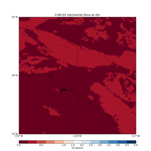
We declare a HorizontalSlice class which specifies a slice between two points, an upper-left point and a bottom-right point, spacing in degrees to query, and the velocity model. We then can say to show the plot by issuing the plot command.
For example, to show a plot of CVM-S5, spaced at 0.01 degrees, from -119,35 to -117,33 at 0m depth, we would do the following:
Figure 1
from pycvm import *
HorizontalSlice(Point(-119,35,0), Point(-117,33,0), 0.01, "cvms5").plot("vs")
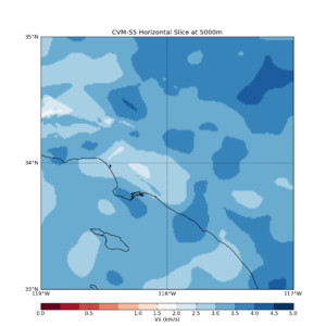
To generate at 5000m depth, we can do the following:
Figure 2
HorizontalSlice(Point(-119,35,5000), Point(-117,33,5000), 0.01, "cvms5").plot("vs")
Please note that the depth is controlled by the first point's depth. Therefore in the above code, the Point(-119,35,5000) class is what specifies that the horizontal slice will be at 5000m depth.
Differencing Horizontal Slices
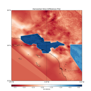
The Difference class allows us to see the difference between two horizontal slices of the same width and height. This allows us to see changes over depth or across velocity models.
For example, suppose we were interested in knowing where the material properties were softer in CVM-S5 at the surface than in CVM-S4. We could do the following:
Figure 3
from pycvm import *
Difference(HorizontalSlice(Point(-120,36,0), Point(-116,32,0), 0.01, "cvms5"), HorizontalSlice(Point(-120,36,0), Point(-116,32,0), 0.01, "cvms")).plot("vs")
Note that the Difference class will take any two horizontal slices or cross sections. So, we can use the class to see where velocity inversions happen as well:
Difference(HorizontalSlice(Point(-120,36,10000), Point(-116,32,10000), 0.01, "cvms5"), HorizontalSlice(Point(-120,36,15000), Point(-116,32,15000), 0.01, "cvms")).plot("vs")
Getting Vs30 Maps
Vs30Slice(Point(-120,36,0), Point(-116,32,0), 0.01, "cvms5").plot()
Because all classes containing "Slice" in them inherit from HorizontalSlice, we can difference Vs30Slice's as well,
Difference(Vs30Slice(Point(-120,36,0), Point(-116,32,0), 0.01, "cvms5"), Vs30Slice(Point(-120,36,0), Point(-116,32,0), 0.01, "cvms")).plot("vs")


