Difference between revisions of "High Frequency CyberShake"
| (36 intermediate revisions by the same user not shown) | |||
| Line 1: | Line 1: | ||
| + | = Cost = | ||
| − | + | The cost to calculate an initial 1 Hz hazard curve for WNGC, with SGTs on Titan and post-processing on Blue Waters, was 230K SUs, broken down as follows: | |
| − | + | *SGT workflow: 40k SUs (17%) | |
| + | **GPU SGTs: 39K SUs (17%) | ||
| + | *PP workflow: 190K SUs (83%) | ||
| + | **Extraction: 88K SUs (39%) | ||
| + | **Synthesis: 101K SUs (44%) | ||
| − | [[File:Comparison of 1000m and 200m runs.png| | + | = Rupture Generation code (genslip v3.3.1) = |
| + | |||
| + | [[File:Comparison of 1000m and 200m runs.png|thumb|left|400px|Figure 1<br/>Green = Run_ID 2465: 1000m SGTs, 1000m synth;<br/> | ||
| + | Magenta = Run_ID 2503: 200m SGTs, 200m synth;<br/> | ||
| + | Orange = Run_ID 2504: 1000m SGTs, 200m synth (interpolation);<br/> | ||
| + | Cyan = Run_ID 2507: 200m SGTs, 1000m synth (most points ignored)]] | ||
| + | |||
| + | To move to higher frequencies, the rupture geometries must have a denser grid spacing, from 1000m for 0.5 Hz to 200 m for 1.0 Hz. We adopted genslip v3.3.1 to resolve an issue in which, since the dimensions of the rupture surfaces can vary a bit going from 1000m to 200m, some ruptures went from 8 rupture variations to 2, resulting in undersampling the rupture and causing artificially large ground motions (Figure 1; magenta curve, compared to green and cyan). Figure 1 illustrates that the issues is related to the resolution of the fault surfaces used in the synthesis, not the resolution the SGTs are saved at. | ||
| + | |||
| + | To address this issue, we moved to genslip v3.3.1, which has the following modifications: | ||
| + | |||
| + | #Wavenumber filter modified so that tall skinny faults (short along strike, long down-dip like Puente Hills) don’t have strong horizontal striping pattern. | ||
| + | #Added stochastic perturbations for rupture initiation time and rise time about median value (V3.2 just used median value). | ||
| + | #Added built-in adjustment of rise time for dipping reverse faults (alphaT parameter of GP2010). | ||
| + | #Added option to self generate the random number seed based on fault dimensions, magnitude and fault location. | ||
| + | #Added option for hypocenter location to be randomly generated within code. Hypocenter can lie anywhere within fault plane, however, the probability is highest in the center and tapers linearly towards the edges. Parameters controlling the probability tapering can be provided by input or just left unspecified for default values. | ||
| + | #For random hypo centers and ERF input (like CyberShake), the number of realizations is determined using a relation that is proportional to fault area. Note that each realization has a unique combination of hypocenter and slip distribution (as opposed to previous version which had multiple slip models for each hypocenter. The formula for specifying the number of realizations is: | ||
| + | |||
| + | Nreal = C * Area / 10.0 | ||
| + | |||
| + | where by default C=0.5. With a standard Mag/Area relation of M=log10(A)+4, this formula gives about 5,50,500 realizations for Mw=6,7,8, respectively. However, I’ve also limited the minimum number of realizations to be 10, so even a Mw=6 will get 10. | ||
| + | |||
| + | This seems to have resolved the issue, as can be seen in a comparison plot of the 1000m and 200m results for the TEST site (Figure 2). Notice they visually match the cyan and green curves in the first plot, as well. | ||
| + | |||
| + | [[File:genslip_v3.3.1a TEST 1000m vs 200m.png|thumb|400px|left|Figure 2]] | ||
| + | |||
| + | == Random vs uniform hypocenter distribution == | ||
| + | |||
| + | [[File:Comparison of hypocenter distributions 3sec.png|thumb|400px|Figure 3<br\>3 sec SA for WNGC. Black is random, purple is uniform.]] | ||
| + | |||
| + | [[File:Comparison of hypocenter distributions 5sec.png|thumb|400px|Figure 4<br\>5 sec SA for WNGC. Black is random, purple is uniform.]] | ||
| + | |||
| + | [[File:Comparison of hypocenter distributions 10sec.png|thumb|400px|Figure 5<br\>10 sec SA for WNGC. Black is random, purple is uniform.]] | ||
| + | |||
| + | We conducted an experiment to see what the impact of random vs uniform hypocenter distribution is on hazard curves. Plots comparing run 3847 (random) to run 3837 (uniform) are in Figures 3-5. | ||
| + | |||
| + | == Optimizations == | ||
| + | |||
| + | Reference problem: 2 rupture variations of source 128, rupture 1296 takes 5m48.195s when compiled with icc -O3 -xhost on Stampede using 1000m spacing. | ||
| + | |||
| + | * Replaced bubble sort of sort_rake with qsort call: 0m25.547s (92.3% improvement) | ||
| + | * Replaced fourg FFT with FFTW FFT, copied data over to FFTW structures: 0m23.045s (9.8% incremental improvement, 93.4% cumulative) | ||
| + | * Removed sort entirely, since median is no longer used: 0m23.140s (0.4% worse, probably noise) | ||
| + | |||
| + | = Seismogram synthesis code = | ||
| + | |||
| + | == Batching for 1 Hz == | ||
| + | |||
| + | [[File:Verification of SeisPSA_lm_multi 3sec.png|thumb|left|400px|Figure 6]] | ||
| + | |||
| + | We took the batching capability from SeisPSA_multi and integrated it into the large memory version for 1 Hz calculations, producing SeisPSA_lm_multi. In this way we can batch our 1 Hz post-processing, reducing the input I/O by a factor equal to the batching factor. | ||
| + | |||
| + | We verified this code by comparing run 3845 (PAS, 0.5 Hz, ERF 35) to run 2722 (PAS, 0.5 Hz, ERF 35) (Figure 6). | ||
| + | |||
| + | == Optimizations == | ||
| + | |||
| + | Reference problem: WNGC, source 86, rupture 6, rupture variation 92 takes 15m11.722s when compiled using icc -O3 on Stampede. | ||
| + | |||
| + | * TODO: Replace get_master_list with get_master_list_opt from 1 Hz extract SGT code | ||
| + | * TODO: Replace find_sgt linear search with binary search | ||
| + | * Tried replacing time-domain convolution with frequency convolution using FFTW. Ended up being 33% slower. I kept the capability in as a flag, as it may be useful later since we could calculate the FFT once, then perform multiple convolutions for different rupture variations. | ||
| + | |||
| + | = RotD calculations = | ||
| + | |||
| + | [[File:Verification of RotD code 3sec.png|thumb|left|400px|Figure 7]] | ||
| + | |||
| + | As the UGMS would like to see RTGM results which use RotD100, we integrated the RotD code into SeisPSA_lm_multi as an optional flag. We verified this by comparing the RotD100 curves from run 3845 (PAS, 0.5 Hz, ERF 35, RotD) to run 2722 (PAS, 0.5 Hz, no RotD) (Figure 7). | ||
Latest revision as of 21:34, 2 December 2014
Contents
Cost
The cost to calculate an initial 1 Hz hazard curve for WNGC, with SGTs on Titan and post-processing on Blue Waters, was 230K SUs, broken down as follows:
- SGT workflow: 40k SUs (17%)
- GPU SGTs: 39K SUs (17%)
- PP workflow: 190K SUs (83%)
- Extraction: 88K SUs (39%)
- Synthesis: 101K SUs (44%)
Rupture Generation code (genslip v3.3.1)
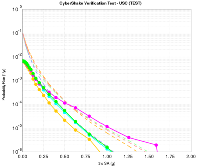
To move to higher frequencies, the rupture geometries must have a denser grid spacing, from 1000m for 0.5 Hz to 200 m for 1.0 Hz. We adopted genslip v3.3.1 to resolve an issue in which, since the dimensions of the rupture surfaces can vary a bit going from 1000m to 200m, some ruptures went from 8 rupture variations to 2, resulting in undersampling the rupture and causing artificially large ground motions (Figure 1; magenta curve, compared to green and cyan). Figure 1 illustrates that the issues is related to the resolution of the fault surfaces used in the synthesis, not the resolution the SGTs are saved at.
To address this issue, we moved to genslip v3.3.1, which has the following modifications:
- Wavenumber filter modified so that tall skinny faults (short along strike, long down-dip like Puente Hills) don’t have strong horizontal striping pattern.
- Added stochastic perturbations for rupture initiation time and rise time about median value (V3.2 just used median value).
- Added built-in adjustment of rise time for dipping reverse faults (alphaT parameter of GP2010).
- Added option to self generate the random number seed based on fault dimensions, magnitude and fault location.
- Added option for hypocenter location to be randomly generated within code. Hypocenter can lie anywhere within fault plane, however, the probability is highest in the center and tapers linearly towards the edges. Parameters controlling the probability tapering can be provided by input or just left unspecified for default values.
- For random hypo centers and ERF input (like CyberShake), the number of realizations is determined using a relation that is proportional to fault area. Note that each realization has a unique combination of hypocenter and slip distribution (as opposed to previous version which had multiple slip models for each hypocenter. The formula for specifying the number of realizations is:
Nreal = C * Area / 10.0
where by default C=0.5. With a standard Mag/Area relation of M=log10(A)+4, this formula gives about 5,50,500 realizations for Mw=6,7,8, respectively. However, I’ve also limited the minimum number of realizations to be 10, so even a Mw=6 will get 10.
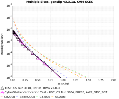
This seems to have resolved the issue, as can be seen in a comparison plot of the 1000m and 200m results for the TEST site (Figure 2). Notice they visually match the cyan and green curves in the first plot, as well.
Random vs uniform hypocenter distribution
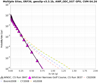
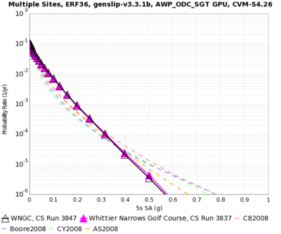
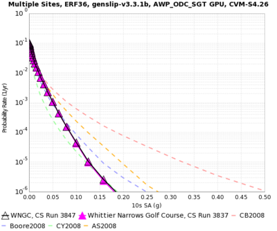
We conducted an experiment to see what the impact of random vs uniform hypocenter distribution is on hazard curves. Plots comparing run 3847 (random) to run 3837 (uniform) are in Figures 3-5.
Optimizations
Reference problem: 2 rupture variations of source 128, rupture 1296 takes 5m48.195s when compiled with icc -O3 -xhost on Stampede using 1000m spacing.
- Replaced bubble sort of sort_rake with qsort call: 0m25.547s (92.3% improvement)
- Replaced fourg FFT with FFTW FFT, copied data over to FFTW structures: 0m23.045s (9.8% incremental improvement, 93.4% cumulative)
- Removed sort entirely, since median is no longer used: 0m23.140s (0.4% worse, probably noise)
Seismogram synthesis code
Batching for 1 Hz
We took the batching capability from SeisPSA_multi and integrated it into the large memory version for 1 Hz calculations, producing SeisPSA_lm_multi. In this way we can batch our 1 Hz post-processing, reducing the input I/O by a factor equal to the batching factor.
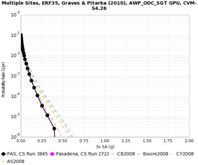
We verified this code by comparing run 3845 (PAS, 0.5 Hz, ERF 35) to run 2722 (PAS, 0.5 Hz, ERF 35) (Figure 6).
Optimizations
Reference problem: WNGC, source 86, rupture 6, rupture variation 92 takes 15m11.722s when compiled using icc -O3 on Stampede.
- TODO: Replace get_master_list with get_master_list_opt from 1 Hz extract SGT code
- TODO: Replace find_sgt linear search with binary search
- Tried replacing time-domain convolution with frequency convolution using FFTW. Ended up being 33% slower. I kept the capability in as a flag, as it may be useful later since we could calculate the FFT once, then perform multiple convolutions for different rupture variations.
RotD calculations
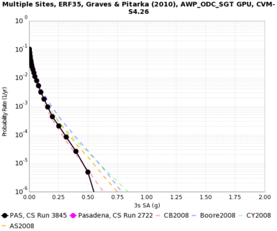
As the UGMS would like to see RTGM results which use RotD100, we integrated the RotD code into SeisPSA_lm_multi as an optional flag. We verified this by comparing the RotD100 curves from run 3845 (PAS, 0.5 Hz, ERF 35, RotD) to run 2722 (PAS, 0.5 Hz, no RotD) (Figure 7).
