Difference between revisions of "Rupture Variation Generator v5.4.2"
| (56 intermediate revisions by the same user not shown) | |||
| Line 4: | Line 4: | ||
== Status == | == Status == | ||
| + | |||
| + | The work below was performed on Summit. | ||
*Replicate reference SRFs using stand-alone code: <span style="color:green">Complete</span> | *Replicate reference SRFs using stand-alone code: <span style="color:green">Complete</span> | ||
*Create RupGen-api-5.4.2: <span style="color:green">Complete</span> | *Create RupGen-api-5.4.2: <span style="color:green">Complete</span> | ||
*Replicate SRFs from stand-alone code using RupGen library: <span style="color:green">Complete</span> | *Replicate SRFs from stand-alone code using RupGen library: <span style="color:green">Complete</span> | ||
| − | *Compile DirectSynth against RupGen library: <span style="color: | + | *Compile DirectSynth against RupGen library: <span style="color:green">Complete<span> |
| − | *Replicate SRFs from stand-alone code using DirectSynth: <span style="color: | + | *Replicate SRFs from stand-alone code using DirectSynth: <span style="color:green">Complete</span> |
| − | *In the database, create new Rupture Variation Scenario ID and populate the Rupture Variations table: <span style="color: | + | *In the database, create new Rupture Variation Scenario ID and populate the Rupture Variations table: <span style="color:#ddcc00">In progress</span> |
| − | *Perform CyberShake run for USC using RupGen-api-5.4.2: <span style="color: | + | *Perform CyberShake run for USC using RupGen-api-5.4.2: <span style="color:green">Complete</span> |
== Verification == | == Verification == | ||
| Line 29: | Line 31: | ||
==== Source 76, rupture 0 ==== | ==== Source 76, rupture 0 ==== | ||
| − | We generated all 77 rupture variations using the stand-alone code, then generated them using test code compiled against the library. | + | We generated all 77 rupture variations using the stand-alone code, then generated them using test code compiled against the library. These were all done on a login node. |
Only a few non-slip fields differed more than the permitted tolerance, less than 1 per variation. | Only a few non-slip fields differed more than the permitted tolerance, less than 1 per variation. | ||
| − | The average difference (which is mostly the difference between slips) was 0.0012%, and the largest difference was ~1e-5 (on values which range up to ~100). | + | The average largest percent difference (which is mostly the difference between slips) was 0.0012%, and the average largest difference was ~1e-5 (on values which range up to ~100). |
Since in the past we have had issues with an order dependence in the rupture generator, we also spot-checked by generating every 10th variation using the test code. These yielded the same md5sums as when they were generated in order. | Since in the past we have had issues with an order dependence in the rupture generator, we also spot-checked by generating every 10th variation using the test code. These yielded the same md5sums as when they were generated in order. | ||
| Line 39: | Line 41: | ||
==== Source 128, rupture 858 ==== | ==== Source 128, rupture 858 ==== | ||
| − | We generated all 256 rupture variations using the stand-alone code, then generated them using test code compiled against the library. | + | We generated all 256 rupture variations using the stand-alone code, then generated them using test code compiled against the library. These were all done on a login node. |
Each rupture variation has approximately 6 differences outside of the tolerance values (out of approximately 2.5 million values). | Each rupture variation has approximately 6 differences outside of the tolerance values (out of approximately 2.5 million values). | ||
| − | The average difference (which is mostly the difference between slips) was 0.0072%, and the largest difference was ~7e-5 (on values which range up to ~1000). | + | The average largest percent difference (which is mostly the difference between slips) was 0.0072%, and the average largest difference was ~7e-5 (on values which range up to ~1000). |
Since in the past we have had issues with an order dependence in the rupture generator, we also spot-checked by generating every 20th variation using the test code. These yielded the same md5sums as when they were generated in order, as did rupture variations 250 and 251 generated consecutively. | Since in the past we have had issues with an order dependence in the rupture generator, we also spot-checked by generating every 20th variation using the test code. These yielded the same md5sums as when they were generated in order, as did rupture variations 250 and 251 generated consecutively. | ||
| Line 56: | Line 58: | ||
Each rupture variation has approximately 498 differences outside of the tolerance values (out of approximately 35 million values). | Each rupture variation has approximately 498 differences outside of the tolerance values (out of approximately 35 million values). | ||
| − | The average difference (which is mostly the difference between slips) was 0.052%, and the largest difference was ~4e-4 (on values which range up to ~10000). | + | The average largest percent difference (which is mostly the difference between slips) was 0.052%, and the average largest difference was ~4e-4 (on values which range up to ~10000). |
The spot-check test was done on rupture variations 0, 10, 20, 30, and 40. We also spot-checked 100, 150, 200, 250, 300, 350, and 400 against the reference, with similar differences. | The spot-check test was done on rupture variations 0, 10, 20, 30, and 40. We also spot-checked 100, 150, 200, 250, 300, 350, and 400 against the reference, with similar differences. | ||
| + | |||
| + | === DirectSynth compiled with librupgen compared with stand-alone code === | ||
| + | |||
| + | For this comparison, we recalculated the stand-alone code results using a compute node, since we saw that this introduces some slight differences, and DirectSynth has to be run on a login node. | ||
| + | |||
| + | ==== Source 76, rupture 0 ==== | ||
| + | |||
| + | We compared all 77 rupture variations. | ||
| + | |||
| + | The average largest difference was 4e-5, and average largest percent difference was 0.0032%. | ||
| + | |||
| + | Using the slightly higher difference tolerance (0.000021), we average 1 difference higher than the tolerance per variation. | ||
| + | |||
| + | ==== Source 128, rupture 858 ==== | ||
| + | |||
| + | We compared all 256 rupture variations. | ||
| + | |||
| + | The average largest difference was 6e-5, and average largest percent difference was 0.0044%. | ||
| + | |||
| + | Using the slightly higher difference tolerance (0.000021), we average 12 differences higher than the tolerance per variation. | ||
| + | |||
| + | ==== Source 68, rupture 7 ==== | ||
| + | |||
| + | We compared only the first 40 rupture variations. | ||
| + | |||
| + | The average largest difference was 8e-4, and average largest percent difference was 0.1293%. | ||
| + | |||
| + | Using the slightly higher difference tolerance (0.000021), we average 19,700 differences higher than the tolerance per variation. | ||
| + | |||
| + | Since this is quite a bit worse than the previous comparison, we also did a comparison with the results generated directly from the library, and got about the same results. | ||
| + | |||
| + | == Optimization == | ||
| + | |||
| + | v5.4.2 is approximately 3x slower than v3.3.1, so we investigated optimization. | ||
| + | |||
| + | We are running source 68, rupture 7, rupture variation 0 as our benchmark. We run it 5 times and take the average. | ||
| + | |||
| + | Reference runtime: 69.400300 sec | ||
| + | |||
| + | === Random number generator === | ||
| + | |||
| + | For source 128, rupture 858 (source 68, rupture 7 produced 42GB trace results), Score-P suggests that gaus_rand() and sfrand() are both called an extraordinary number of times and are responsible for about 75% of the runtime (total runtime was 18.9 sec): | ||
| + | |||
| + | <pre> | ||
| + | cube::Region NumberOfCalls ExclusiveTime InclusiveTime | ||
| + | gaus_rand 5531760 8.104156 15.400368 | ||
| + | sfrand 66381120 7.296212 7.296212 | ||
| + | fft2d_fftw 14 1.584906 1.584949 | ||
| + | write_srf2 1 1.272117 1.272618 | ||
| + | kfilt_beta2 2 1.182854 15.778140 | ||
| + | ... | ||
| + | </pre> | ||
| + | |||
| + | Various optimizations on gaus_rand() and sfrand(), and the -mcpu=power9 compiler flag got us about 1% speedup on source 68, rupture 7. | ||
| + | |||
| + | Running Score-P on a larger rupture (source 63, rupture 3) gives a different breakdown, with more time spent in kfilt_beta2 and fft2d_fftw: | ||
| + | |||
| + | <pre> | ||
| + | cube::Region NumberOfCalls ExclusiveTime InclusiveTime | ||
| + | fft2d_fftw 14 7.450708 7.450762 | ||
| + | kfilt_beta2 2 5.281393 8.775227 | ||
| + | write_srf2 1 3.780037 3.780435 | ||
| + | gaus_rand 24231024 3.583294 3.583294 | ||
| + | kfilter 1 0.822850 0.822850 | ||
| + | gen_Mliu_stf 110892 0.365619 0.398298 | ||
| + | _mc_read_ruppars 1 0.197096 0.271803 | ||
| + | mc_genslip 1 0.152591 18.446691 | ||
| + | </pre> | ||
| + | |||
| + | Only about 0.7 sec of the time in fft2d_fftw that's used isn't due to fftw calls, so there's not much potential for optimization. | ||
| + | |||
| + | === kfilt_beta2 === | ||
| + | |||
| + | In kfilt_beta2, about 25% of the time is spent in the if statement which calculates amp. Some refactoring to pull out constants and eliminate as many exp() and log() calls as possible reduced the runtime of this if statement by 75%, yielding an overall improvement of 19%. | ||
| + | |||
| + | Specifically, we took (slip.c, line 1457) | ||
| + | <pre> | ||
| + | k2 = kx*kx + ky*ky; | ||
| + | fac = 1.0/((1.0 + exp(ord*log(k2*lmin2)))*(1.0 + exp(-ord*log(k2*lmax2)))); | ||
| + | amp = fac*exp(-0.5*beta2*log(k2)); | ||
| + | </pre> | ||
| + | |||
| + | and modified it via algebraic manipulation and pulling constants out of the loops: | ||
| + | <pre> | ||
| + | //New constants | ||
| + | float lmin2_ord = pow(lmin2, ord); | ||
| + | float lmax2_neg_ord = pow(lmax2, -1.0*ord); | ||
| + | float k2_ord; | ||
| + | |||
| + | for(j=0;j<=ny0/2;j++) /* only do positive half, then use symmetry */ | ||
| + | <snip> | ||
| + | k2 = kx*kx + ky*ky; | ||
| + | k2_ord = k2*k2*k2*k2; | ||
| + | fac = 1.0/((1.0+k2_ord*lmin2_ord)*(1.0+1.0/k2_ord*lmax2_neg_ord)); | ||
| + | amp = fac*1.0/k2; | ||
| + | </pre> | ||
| + | These optimizations depend on beta=2 and ord=4, so before the for loops I added checks that this is in fact true: | ||
| + | <pre> | ||
| + | if (ord!=4) { | ||
| + | fprintf(stderr, "The optimized calculation of amp in kfilt_beta2 depends on ord=4. Ord is actually %d, so we are aborting and you should change this calculation back to the unoptimized version.\n", ord); | ||
| + | exit(5); | ||
| + | } | ||
| + | |||
| + | if (fabs(beta2-2.0)>0.000001) { | ||
| + | fprintf(stderr, "The optimized calculation of amp in kfilt_beta2 depends on beta2 = 2. beta2 is actually %d, so we are aborting and you should change this calculation.\n", beta2); | ||
| + | exit(6); | ||
| + | } | ||
| + | </pre> | ||
| + | |||
| + | == target_hypo_spacing == | ||
| + | |||
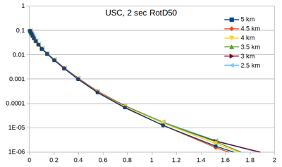
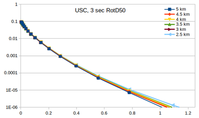
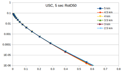
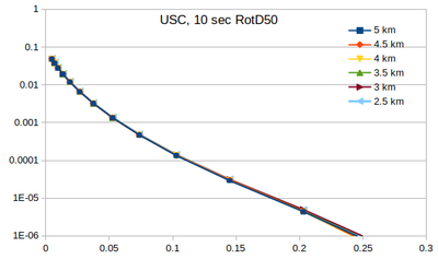
| + | '''Conclusion: ''' we will use 4 km spacing for CyberShake runs using genslip-v5.4.2. Due to sampling effects (more details below), this value may slightly underestimate the hazard at long return periods (>1e-5) | ||
| + | |||
| + | One of the parameters to genslip is 'target_hypo_spacing', which determines the spacing between hypocenters when rupture variations are generated. Decreasing the spacing improves sampling, but also increases the number of rupture variations and increases runtime. Past CyberShake runs used the value 4.5 km. | ||
| + | |||
| + | We performed an experiment in which, for site USC using the Study 15.4 parameters, varied the target_hypo_spacing value from 2.5 km to 5 km in 0.5 km increments, and compared the resulting hazard curves. | ||
| + | |||
| + | The table below shows how many rupture variations were considered for each spacing, and what increase/decrease in post-processing computational cost this represents, compared to the 4.5 km used in the past. | ||
| + | |||
| + | {| border="1" | ||
| + | ! Spacing !! Number of rupture variations !! Change in computational cost | ||
| + | |- | ||
| + | | 5 km || 371,513 || -22% | ||
| + | |- | ||
| + | | 4.5 km || 476,429 || 0% | ||
| + | |- | ||
| + | | 4 km || 623,290 || 31% | ||
| + | |- | ||
| + | | 3.5 km || 793,184 || 66% | ||
| + | |- | ||
| + | | 3 km || 1,135,139 || 138% | ||
| + | |- | ||
| + | | 2.5 km || 1,609,701 || 238% | ||
| + | |} | ||
| + | |||
| + | === Curves === | ||
| + | Below are plots of the RotD50 hazard curves for each spacing, using data from [[:File:target_hypo_spacing_data.ods | this spreadsheet]]. | ||
| + | |||
| + | {| | ||
| + | ! 2 sec RotD50 !! 3 sec RotD50 !! 5 sec RotD50 !! 10 sec RotD50 | ||
| + | |- | ||
| + | | [[File:target_hypo_spacing_2sRotD50_curve_plots.png|left|thumb|400px]] | ||
| + | | [[File:target_hypo_spacing_3sRotD50_curve_plots.png|left|thumb|400px]] | ||
| + | | [[File:target_hypo_spacing_5sRotD50_curve_plots.png|left|thumb|400px]] | ||
| + | | [[File:target_hypo_spacing_10sRotD50_curve_plots.png|left|thumb|400px]] | ||
| + | |} | ||
| + | |||
| + | |||
| + | The highest hazard is in the sparsest spacing at high probabilities and the densest spacing at low probabilities. | ||
| + | |||
| + | === Disaggregation === | ||
| + | |||
| + | We performed disaggregation at 1e-6 for 3 sec RotD50 at the 6 hypocenter spacings. | ||
| + | |||
| + | {|border="1" | ||
| + | ! !! 5 km !! 4.5 km !! 4 km !! 3.5 km !! 3 km !! 2.5 km | ||
| + | |- | ||
| + | ! Top contributor | ||
| + | | source 219 (Newport Inglewood) | ||
| + | 30.21% | ||
| + | | source 244 (Puente Hills (LA)) | ||
| + | 49.66% | ||
| + | | source 244 (Puente Hills (LA)) | ||
| + | 60.88% | ||
| + | | source 244 (Puente Hills (LA)) | ||
| + | 40.20% | ||
| + | | source 244 (Puente Hills (LA)) | ||
| + | 36.90% | ||
| + | | source 244 (Puente Hills (LA)) | ||
| + | 59.47% | ||
| + | |- | ||
| + | ! 2nd | ||
| + | | source 244 (Puente Hills (LA)) | ||
| + | 23.59% | ||
| + | | source 219 (Newport Inglewood) | ||
| + | 20.04% | ||
| + | | source 219 (Newport Inglewood) | ||
| + | 15.81% | ||
| + | | source 219 (Newport Inglewood) | ||
| + | 18.27% | ||
| + | | source 219 (Newport Inglewood) | ||
| + | 17.26% | ||
| + | | source 265 (Santa Monica) | ||
| + | 11.62% | ||
| + | |- | ||
| + | ! 3rd | ||
| + | | source 265 (Santa Monica) | ||
| + | 17.64% | ||
| + | | source 218 (Newport Inglewood) | ||
| + | 13.67% | ||
| + | | source 218 (Newport Inglewood) | ||
| + | 14.25% | ||
| + | | source 218 (Newport Inglewood) | ||
| + | 14.96% | ||
| + | | source 218 (Newport Inglewood) | ||
| + | 16.80% | ||
| + | | source 219 (Newport Inglewood) | ||
| + | 10.95% | ||
| + | |} | ||
| + | |||
| + | === Source 244, rupture 12 === | ||
| + | |||
| + | We pulled out source 244, rupture 12, since rupture 12 was the rupture with the largest ground motions for source 244, and looked at the individual IMs for each spacing. This ranged from 28 rupture variations for the 5 km spacing to 12 variations for the 2.5 km spacing. | ||
| + | |||
| + | Their means and medians look quite similar, but we see a higher max for 3.5 and 2.5 km. | ||
| + | |||
| + | {| border="1" | ||
| + | ! Spacing !! Mean !! Median !! Min !! Max | ||
| + | |- | ||
| + | ! 5 km | ||
| + | | 763.73 || 770.37 || 266.85 || 1470.71 | ||
| + | |- | ||
| + | ! 4.5 km | ||
| + | | 791.63 || 758.99 || 223.47 || 1504.48 | ||
| + | |- | ||
| + | ! 4 km | ||
| + | | 833.84 || 788.58 || 406.21 || 1473.57 | ||
| + | |- | ||
| + | ! 3.5 km | ||
| + | | 801.43 || 765.02 || 346.44 || 1654.31 | ||
| + | |- | ||
| + | ! 3 km | ||
| + | | 793.99 || 742.54 || 426.42 || 1455.13 | ||
| + | |- | ||
| + | ! 2.5 km | ||
| + | | 795.67 || 738.93 || 242.04 || 1856.50 | ||
| + | |} | ||
| + | |||
| + | I created a histogram of the fraction of rupture variations to fall in each IM bin (for 3 sec RotD50). It does look like we have more representation at the high end with the denser spacings. | ||
| + | |||
| + | [[File:target_hypo_spacing_s244_r12_3sRotD50_histogram.png]] | ||
| + | |||
| + | === 5 km with different seeds === | ||
| + | |||
| + | To examine whether the effects seen with different spacings are due to sampling, we ran the post-processing at 5 km 3 more times with different initial seeds, producing 4 different sets of rupture realizations at 5 km spacing. This gives us approximately the same size sample as the 2.5 km spacing. | ||
| + | |||
| + | Below is a histogram comparing the distribution of IMs for 3 sec RotD50 between 1) 5 km spacing; 2) the 4 sets of 5 km spacing with different seeds, taken together as a group; 3) the 2.5 km spacing. The 4 sets of 5 km spacing have a very similar distribution to the 2.5 km spacing, supporting the hypothesis that the larger IMs we are seeing with denser spacing are just due to increased sampling. | ||
| + | |||
| + | [[File:target_hypo_spacing_s244_r12_3sRotD50_multiseed_histogram.png]] | ||
| + | |||
| + | == Comparison with v3.3.1 == | ||
| + | |||
| + | At site USC, there is little difference between the v3.3.1 (in green) and the v5.4.2 hazard curves. | ||
| + | |||
| + | {| | ||
| + | ! 2 sec RotD50 !! 3 sec RotD50 !! 5 sec RotD50 !! 10 sec RotD50 | ||
| + | |- | ||
| + | | [[File:USC_v5.4.2_compare_with_7052_2sec_RotD50.png|thumb|400px]] | ||
| + | | [[File:USC_v5.4.2_compare_with_7052_3sec_RotD50.png|thumb|400px]] | ||
| + | | [[File:USC_v5.4.2_compare_with_7052_5sec_RotD50.png|thumb|400px]] | ||
| + | | [[File:USC_v5.4.2_compare_with_7052_10sec_RotD50.png|thumb|400px]] | ||
| + | |} | ||
Latest revision as of 18:25, 31 October 2022
This page details the work to migrate the Graves & Pitarka (2019) rupture generator, v5.4.2, to CyberShake.
The specific code changes required to create an API are detailed here: Rupture Variation Generator v5.4.2 code changes
Status
The work below was performed on Summit.
- Replicate reference SRFs using stand-alone code: Complete
- Create RupGen-api-5.4.2: Complete
- Replicate SRFs from stand-alone code using RupGen library: Complete
- Compile DirectSynth against RupGen library: Complete
- Replicate SRFs from stand-alone code using DirectSynth: Complete
- In the database, create new Rupture Variation Scenario ID and populate the Rupture Variations table: In progress
- Perform CyberShake run for USC using RupGen-api-5.4.2: Complete
Verification
The verification sequence is:
- Reference results from Rob
- (1) reproduced using Rob's supplied stand-alone code, compiled and run on a Summit head node.
- (2) is used to produce reference SRFs from ERF 36 geometry files for
- Source 76, rupture 0 (M6.35)
- Source 128, rupture 858 (M7.35)
- Source 68, rupture 7 (M8.45)
- Results from (3) are reproduced using test code which is compiled against the RupGen-api-5.4.2 library.
- Results from (3) are reproduced using DirectSynth and writing out the SRFs.
RupGen-api-5.4.2 against stand-alone code
Source 76, rupture 0
We generated all 77 rupture variations using the stand-alone code, then generated them using test code compiled against the library. These were all done on a login node.
Only a few non-slip fields differed more than the permitted tolerance, less than 1 per variation.
The average largest percent difference (which is mostly the difference between slips) was 0.0012%, and the average largest difference was ~1e-5 (on values which range up to ~100).
Since in the past we have had issues with an order dependence in the rupture generator, we also spot-checked by generating every 10th variation using the test code. These yielded the same md5sums as when they were generated in order.
Source 128, rupture 858
We generated all 256 rupture variations using the stand-alone code, then generated them using test code compiled against the library. These were all done on a login node.
Each rupture variation has approximately 6 differences outside of the tolerance values (out of approximately 2.5 million values).
The average largest percent difference (which is mostly the difference between slips) was 0.0072%, and the average largest difference was ~7e-5 (on values which range up to ~1000).
Since in the past we have had issues with an order dependence in the rupture generator, we also spot-checked by generating every 20th variation using the test code. These yielded the same md5sums as when they were generated in order, as did rupture variations 250 and 251 generated consecutively.
Source 68, rupture 7
All these SRFs were generated on the compute nodes. If you generate them on a login node, you will get something slightly different.
This source/rupture combo has 1190 rupture variations, but since each one takes about 90 seconds to generate, it would take 30 hours to create them all. Instead, we used the stand-alone code to generate the first 423 rupture variations, then generated the first 41 using test code compiled against the library.
Using the same tolerances, many rupture variations had more than 10% of points which at least 1 difference, which causes an abort. We doubled the tolerance (from 0.00011 to 0.00021) and ran the comparisons again. Each rupture variation has approximately 498 differences outside of the tolerance values (out of approximately 35 million values).
The average largest percent difference (which is mostly the difference between slips) was 0.052%, and the average largest difference was ~4e-4 (on values which range up to ~10000).
The spot-check test was done on rupture variations 0, 10, 20, 30, and 40. We also spot-checked 100, 150, 200, 250, 300, 350, and 400 against the reference, with similar differences.
DirectSynth compiled with librupgen compared with stand-alone code
For this comparison, we recalculated the stand-alone code results using a compute node, since we saw that this introduces some slight differences, and DirectSynth has to be run on a login node.
Source 76, rupture 0
We compared all 77 rupture variations.
The average largest difference was 4e-5, and average largest percent difference was 0.0032%.
Using the slightly higher difference tolerance (0.000021), we average 1 difference higher than the tolerance per variation.
Source 128, rupture 858
We compared all 256 rupture variations.
The average largest difference was 6e-5, and average largest percent difference was 0.0044%.
Using the slightly higher difference tolerance (0.000021), we average 12 differences higher than the tolerance per variation.
Source 68, rupture 7
We compared only the first 40 rupture variations.
The average largest difference was 8e-4, and average largest percent difference was 0.1293%.
Using the slightly higher difference tolerance (0.000021), we average 19,700 differences higher than the tolerance per variation.
Since this is quite a bit worse than the previous comparison, we also did a comparison with the results generated directly from the library, and got about the same results.
Optimization
v5.4.2 is approximately 3x slower than v3.3.1, so we investigated optimization.
We are running source 68, rupture 7, rupture variation 0 as our benchmark. We run it 5 times and take the average.
Reference runtime: 69.400300 sec
Random number generator
For source 128, rupture 858 (source 68, rupture 7 produced 42GB trace results), Score-P suggests that gaus_rand() and sfrand() are both called an extraordinary number of times and are responsible for about 75% of the runtime (total runtime was 18.9 sec):
cube::Region          NumberOfCalls ExclusiveTime InclusiveTime
gaus_rand                   5531760      8.104156     15.400368
sfrand                     66381120      7.296212      7.296212
fft2d_fftw                       14      1.584906      1.584949
write_srf2                        1      1.272117      1.272618
kfilt_beta2                       2      1.182854     15.778140
...
Various optimizations on gaus_rand() and sfrand(), and the -mcpu=power9 compiler flag got us about 1% speedup on source 68, rupture 7.
Running Score-P on a larger rupture (source 63, rupture 3) gives a different breakdown, with more time spent in kfilt_beta2 and fft2d_fftw:
cube::Region          NumberOfCalls ExclusiveTime InclusiveTime
fft2d_fftw                       14      7.450708      7.450762
kfilt_beta2                       2      5.281393      8.775227
write_srf2                        1      3.780037      3.780435
gaus_rand                  24231024      3.583294      3.583294
kfilter                           1      0.822850      0.822850
gen_Mliu_stf                 110892      0.365619      0.398298
_mc_read_ruppars                  1      0.197096      0.271803
mc_genslip                        1      0.152591     18.446691
Only about 0.7 sec of the time in fft2d_fftw that's used isn't due to fftw calls, so there's not much potential for optimization.
kfilt_beta2
In kfilt_beta2, about 25% of the time is spent in the if statement which calculates amp. Some refactoring to pull out constants and eliminate as many exp() and log() calls as possible reduced the runtime of this if statement by 75%, yielding an overall improvement of 19%.
Specifically, we took (slip.c, line 1457)
k2 = kx*kx + ky*ky;
fac = 1.0/((1.0 + exp(ord*log(k2*lmin2)))*(1.0 + exp(-ord*log(k2*lmax2))));
amp = fac*exp(-0.5*beta2*log(k2));
and modified it via algebraic manipulation and pulling constants out of the loops:
//New constants
float lmin2_ord = pow(lmin2, ord);
float lmax2_neg_ord = pow(lmax2, -1.0*ord);
float k2_ord;

for(j=0;j<=ny0/2;j++)  /* only do positive half, then use symmetry */
<snip>
        k2 = kx*kx + ky*ky;
        k2_ord = k2*k2*k2*k2;
        fac = 1.0/((1.0+k2_ord*lmin2_ord)*(1.0+1.0/k2_ord*lmax2_neg_ord));
        amp = fac*1.0/k2;
These optimizations depend on beta=2 and ord=4, so before the for loops I added checks that this is in fact true:
if (ord!=4) {
        fprintf(stderr, "The optimized calculation of amp in kfilt_beta2 depends on ord=4.  Ord is actually %d, so we are aborting and you should change this calculation back to the unoptimized version.\n", ord);
        exit(5);
}

if (fabs(beta2-2.0)>0.000001) {
        fprintf(stderr, "The optimized calculation of amp in kfilt_beta2 depends on beta2 = 2.  beta2 is actually %d, so we are aborting and you should change this calculation.\n", beta2);
        exit(6);
}
target_hypo_spacing
Conclusion: we will use 4 km spacing for CyberShake runs using genslip-v5.4.2. Due to sampling effects (more details below), this value may slightly underestimate the hazard at long return periods (>1e-5)
One of the parameters to genslip is 'target_hypo_spacing', which determines the spacing between hypocenters when rupture variations are generated. Decreasing the spacing improves sampling, but also increases the number of rupture variations and increases runtime. Past CyberShake runs used the value 4.5 km.
We performed an experiment in which, for site USC using the Study 15.4 parameters, varied the target_hypo_spacing value from 2.5 km to 5 km in 0.5 km increments, and compared the resulting hazard curves.
The table below shows how many rupture variations were considered for each spacing, and what increase/decrease in post-processing computational cost this represents, compared to the 4.5 km used in the past.
| Spacing | Number of rupture variations | Change in computational cost |
|---|---|---|
| 5 km | 371,513 | -22% |
| 4.5 km | 476,429 | 0% |
| 4 km | 623,290 | 31% |
| 3.5 km | 793,184 | 66% |
| 3 km | 1,135,139 | 138% |
| 2.5 km | 1,609,701 | 238% |
Curves
Below are plots of the RotD50 hazard curves for each spacing, using data from this spreadsheet.
| 2 sec RotD50 | 3 sec RotD50 | 5 sec RotD50 | 10 sec RotD50 |
|---|---|---|---|
The highest hazard is in the sparsest spacing at high probabilities and the densest spacing at low probabilities.
Disaggregation
We performed disaggregation at 1e-6 for 3 sec RotD50 at the 6 hypocenter spacings.
| 5 km | 4.5 km | 4 km | 3.5 km | 3 km | 2.5 km | |
|---|---|---|---|---|---|---|
| Top contributor | source 219 (Newport Inglewood)
30.21% |
source 244 (Puente Hills (LA))
49.66% |
source 244 (Puente Hills (LA))
60.88% |
source 244 (Puente Hills (LA))
40.20% |
source 244 (Puente Hills (LA))
36.90% |
source 244 (Puente Hills (LA))
59.47% |
| 2nd | source 244 (Puente Hills (LA))
23.59% |
source 219 (Newport Inglewood)
20.04% |
source 219 (Newport Inglewood)
15.81% |
source 219 (Newport Inglewood)
18.27% |
source 219 (Newport Inglewood)
17.26% |
source 265 (Santa Monica)
11.62% |
| 3rd | source 265 (Santa Monica)
17.64% |
source 218 (Newport Inglewood)
13.67% |
source 218 (Newport Inglewood)
14.25% |
source 218 (Newport Inglewood)
14.96% |
source 218 (Newport Inglewood)
16.80% |
source 219 (Newport Inglewood)
10.95% |
Source 244, rupture 12
We pulled out source 244, rupture 12, since rupture 12 was the rupture with the largest ground motions for source 244, and looked at the individual IMs for each spacing. This ranged from 28 rupture variations for the 5 km spacing to 12 variations for the 2.5 km spacing.
Their means and medians look quite similar, but we see a higher max for 3.5 and 2.5 km.
| Spacing | Mean | Median | Min | Max |
|---|---|---|---|---|
| 5 km | 763.73 | 770.37 | 266.85 | 1470.71 |
| 4.5 km | 791.63 | 758.99 | 223.47 | 1504.48 |
| 4 km | 833.84 | 788.58 | 406.21 | 1473.57 |
| 3.5 km | 801.43 | 765.02 | 346.44 | 1654.31 |
| 3 km | 793.99 | 742.54 | 426.42 | 1455.13 |
| 2.5 km | 795.67 | 738.93 | 242.04 | 1856.50 |
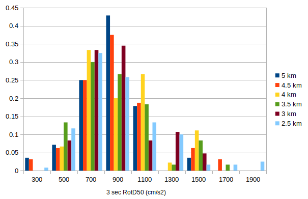
I created a histogram of the fraction of rupture variations to fall in each IM bin (for 3 sec RotD50). It does look like we have more representation at the high end with the denser spacings.
5 km with different seeds
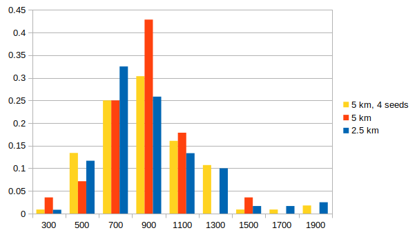
To examine whether the effects seen with different spacings are due to sampling, we ran the post-processing at 5 km 3 more times with different initial seeds, producing 4 different sets of rupture realizations at 5 km spacing. This gives us approximately the same size sample as the 2.5 km spacing.
Below is a histogram comparing the distribution of IMs for 3 sec RotD50 between 1) 5 km spacing; 2) the 4 sets of 5 km spacing with different seeds, taken together as a group; 3) the 2.5 km spacing. The 4 sets of 5 km spacing have a very similar distribution to the 2.5 km spacing, supporting the hypothesis that the larger IMs we are seeing with denser spacing are just due to increased sampling.
Comparison with v3.3.1
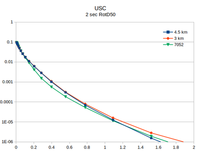
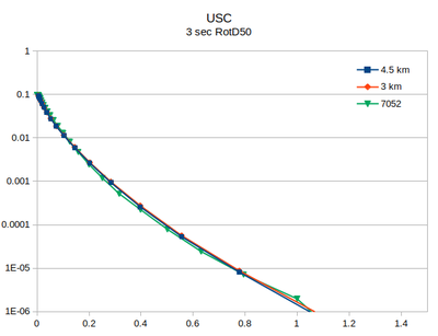
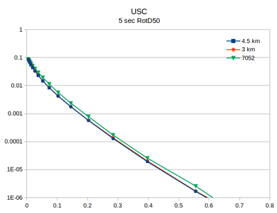
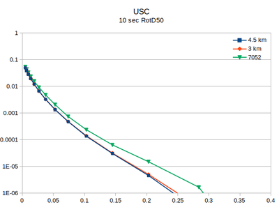
At site USC, there is little difference between the v3.3.1 (in green) and the v5.4.2 hazard curves.
| 2 sec RotD50 | 3 sec RotD50 | 5 sec RotD50 | 10 sec RotD50 |
|---|---|---|---|
