CyberShake Study 22.12

CyberShake Study 22.10 is a proposed study in Southern California which will include deterministic low-frequency (0-1 Hz) and stochastic high-frequency (1-50 Hz) simulations. We will use the Graves & Pitarka (2019) rupture generator and the high frequency modules from the SCEC Broadband Platform v22.4.

Status

This study is in the planning phase. We estimate calculations will begin in October 2022.

Velocity Model

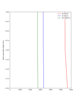
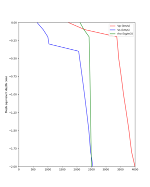
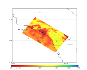
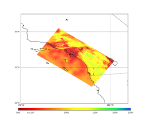
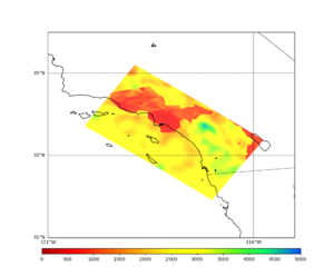
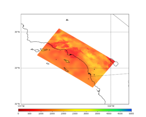
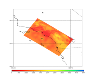
We are planning to use CVM-S4.26 with a GTL applied, and the CVM-S4 1D background model outside of the region boundaries.

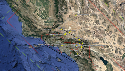
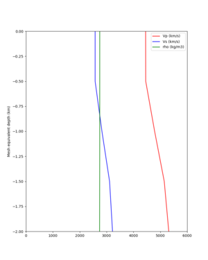
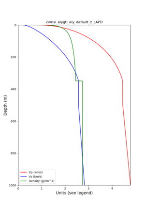
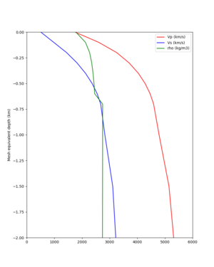
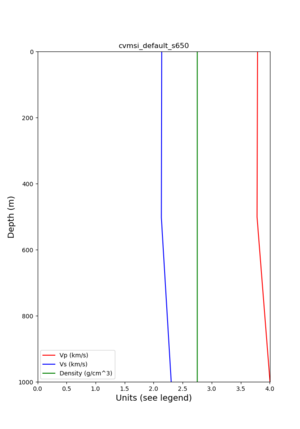
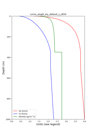
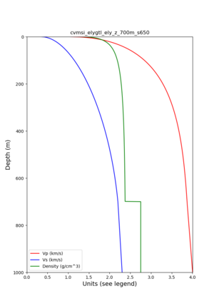
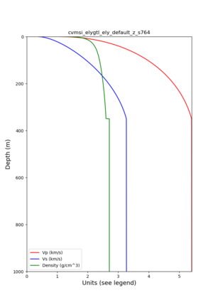
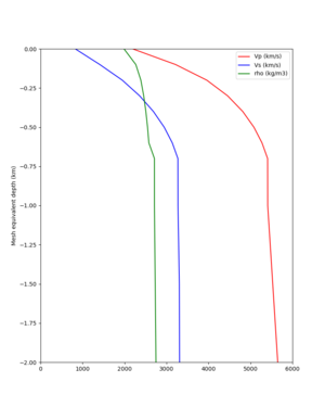
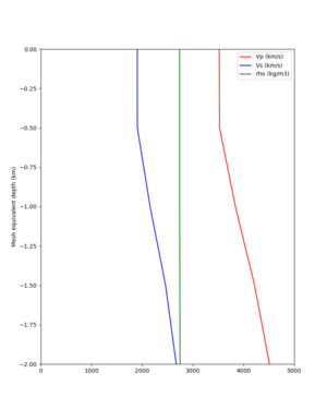
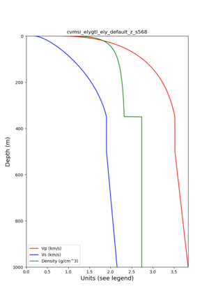
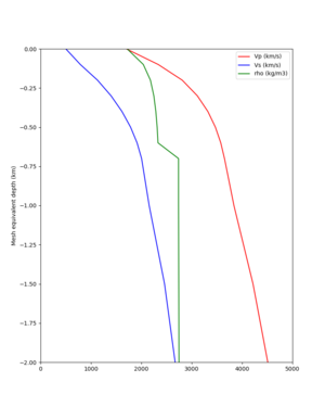
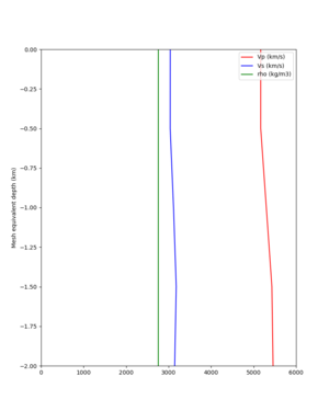
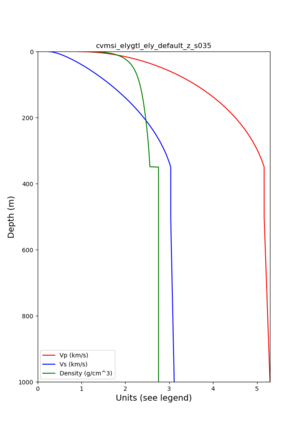
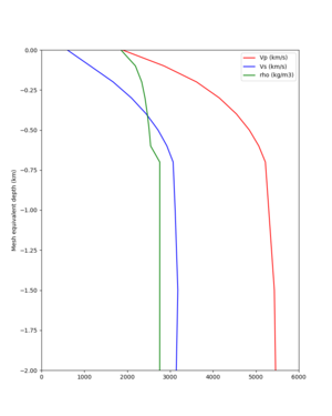
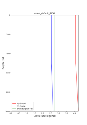
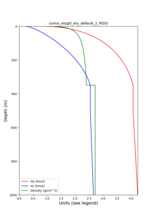
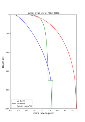
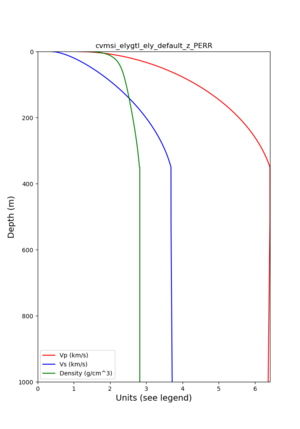
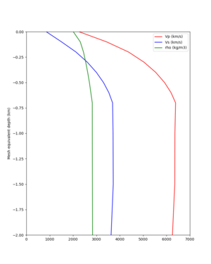
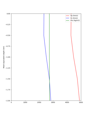
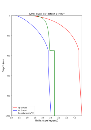
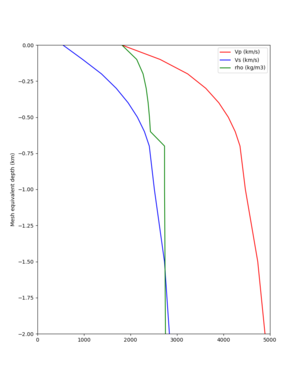
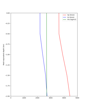
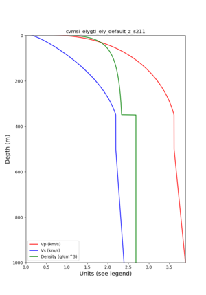
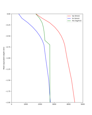
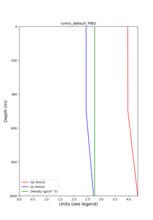
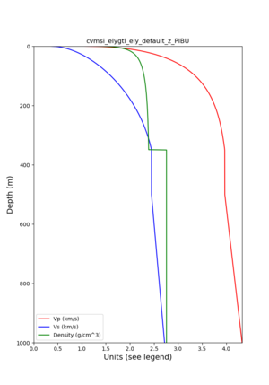
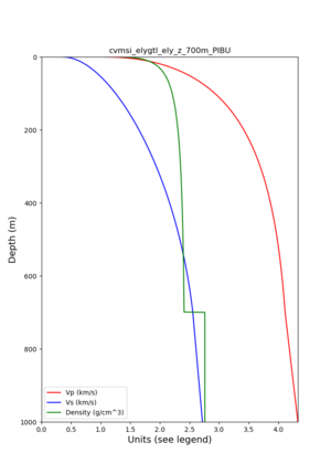
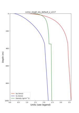
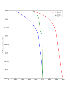
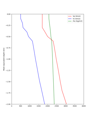
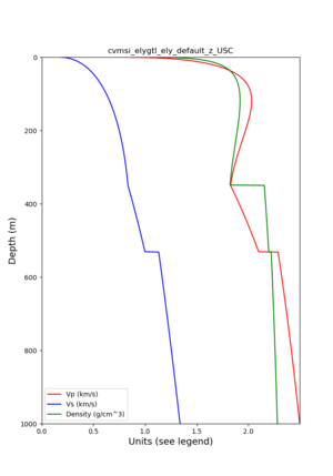
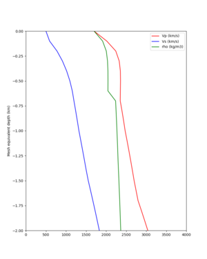
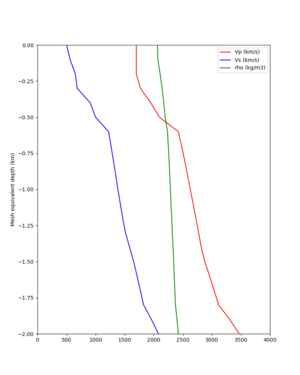
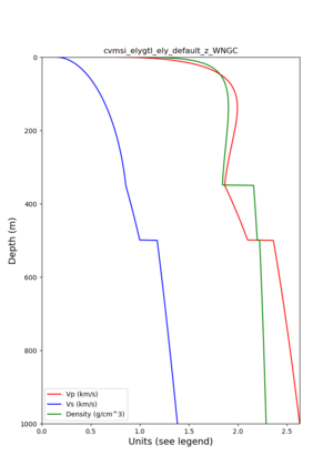
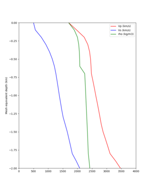
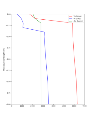
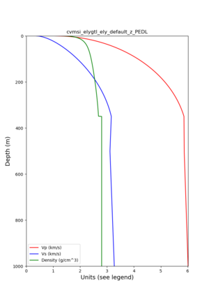
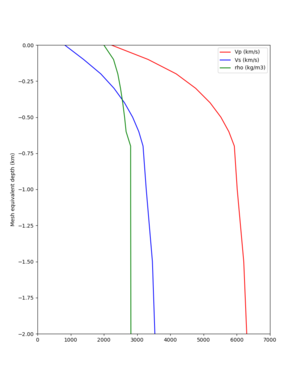
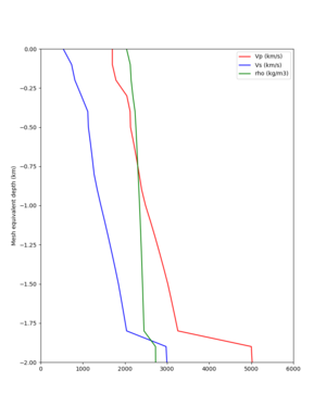
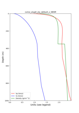
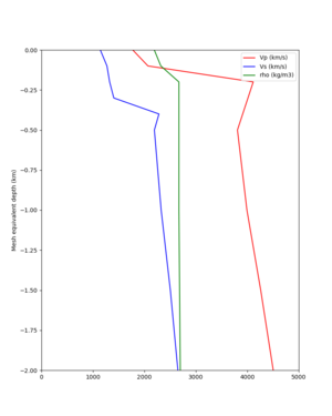
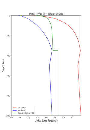
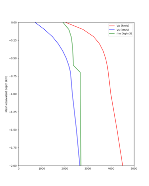
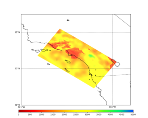
We are investigating applying the Ely-Jordan GTL down to 700 m instead of the default of 350m. We extracted profiles for a series of southern California CyberShake sites, with no GTL, a GTL applied down to 350m, and a GTL applied down to 700m.

Sites (the CVM-S4.26 basins are outlined in red):

These are for sites outside of the CVM-S4.26 basins:

Site	No GTL	350m GTL	700m GTL
LAPD
s650
s764
s568
s035
RIDG
PERR
MRVY
s211
PIBU

These are for sites inside of the CVM-S4.26 basins:

Site	No GTL	350m GTL	700m GTL
s117
USC
WNGC
PEDL
SBSM
SVD

Proposed Algorithm

Our proposed algorithm for generating the velocity model is as follows:

1. Set the surface mesh point to a depth of 25m.
2. Query the CVM-S4.26.M01 model ('cvmsi' string in UCVM) for each grid point.
3. Calculate the Ely taper at that point using 700m as the transition depth.
4. Compare the values before and after the taper modification; at each grid point down to the transition depth, use the value from the method with the lower Vs value.
5. Check values for Vp/Vs ratio, minimum Vs, Inf/NaNs, etc.

Cross-sections

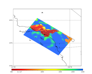
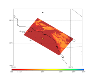
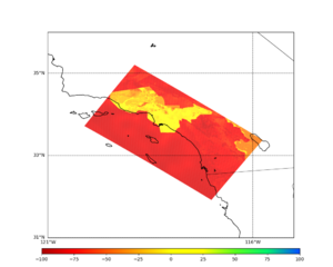
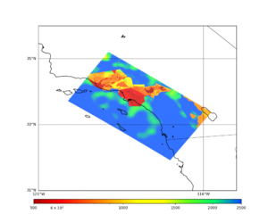
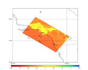
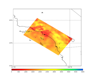
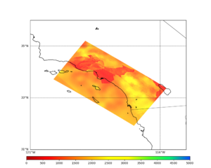
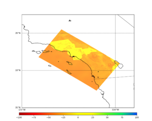
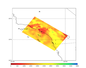
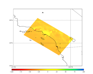
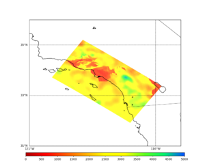
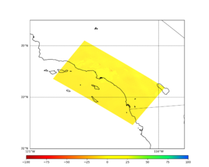
Below are cross-sections of the TEST site velocity model at depths down to 600m for CVM-S4.26.M01, the taper to 700m, the lesser of the two values, and the % difference.

Depth	CVM-S4.26.M01	Ely taper to 700m	Selecting smaller value	% difference
0m (queried at 25m depth)
100m
200m
300m
400m
500m
600m

High-frequency codes

For this study, we will use the Graves & Pitarka high frequency module (hb_high) from the Broadband Platform v22.4, hb_high_v6.0.5. We will use the following parameters. Parameters in bold have been changed for this study.

Parameter	Value
stress_average	50
rayset	2,1,2
siteamp	1
nbu	4 (not used)
ifft	0 (not used)
flol	0.02 (not used)
fhil	19.9 (not used)
irand	Seed used for generating SRF
tlen	Seismogram length, in sec
dt	0.01
fmax	10 (not used)
kappa	0.04
qfexp	0.6
mean_rvfac	0.775
range_rvfac	0.1
rvfac	Calculated using BBP hfsims_cfg.py code
shal_rvfac	0.6
deep_rvfac	0.6
czero	2
c_alpha	-99
sm	-1
vr	-1
vsmoho	999.9
nlskip	-99
vpsig	0
vshsig	0
rhosig	0
qssig	0
icflag	1
velname	-1
fa_sig1	0
fa_sig2	0
rvsig1	0.1
ipdur_model	11
ispar_adjust	1
targ_mag	-1
fault_area	-1
default_c0	57
default_c1	34

Spectral Content around 1 Hz

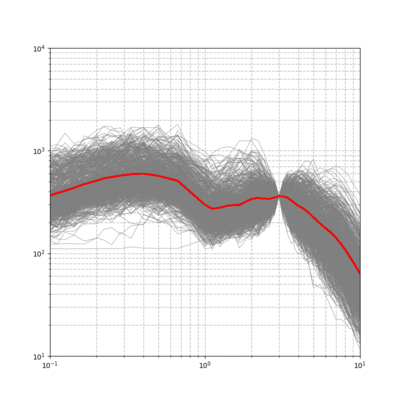
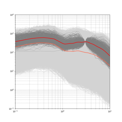
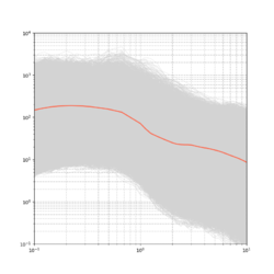
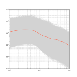
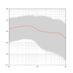
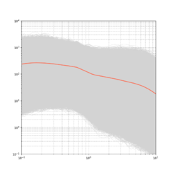
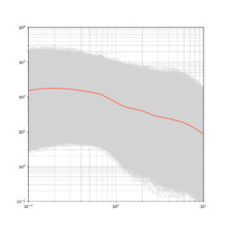
We investigated the spectral content of the Broadband CyberShake results in the 0.5-3 second range, to look for any discontinuities.

The plot below is from WNGC, Study 15.12 (run ID 4293).

Spectral plot for WNGC from Study 15.12, target of 0.3676g @ 3 sec. Mean is in red.

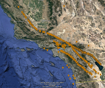
Below is a plot of the hypocenters from the 706 rupture variations which meet the target.

These events have a different distribution than the rupture variations as a whole.

Fault	Percent of target RVs	Percent of all RVs
San Andreas	60	44
Elsinore	21	9
San Jacinto	13	8
Other	6	39

Additionally, 88% of the selected events have a magnitude greater than the average for their source. 4% are average, and 8% are lower.

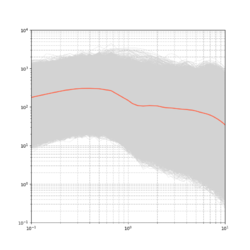
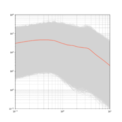
Below is a spectral plot but which includes all rupture variations and the overall mean (in orange).

Spectral plot for WNGC from Study 15.12, all variations.

Additional Sites

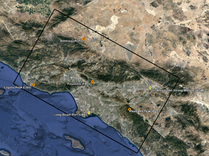
We created spectral plots for 7 additional sites (STNI, SBSM, PAS, LGU, LBP, ALP, PLS), located here:

STNI	SBSM	PAS	LGU	LBP	ALP	PLS

Production Checklist

Science to-dos

• Perform validation for Northridge, Chino Hills, Whittier, Landers, Hector Mine, and North Palm Springs
• For each validation event, calculate BBP results, CS results, and CS results with BBP Vs30 values
• Check for spectral discontinuities around 1 Hz
• Decide if we should stick with rvfrac=0.8 or allow it to vary

• Determine appropriate SGT, low-frequency, and high-frequency seismogram durations
• Update high-frequency Vs30 to use released Thompson values

Technical to-dos

• Integrate refactoring of BBP codes into latest BBP release
• Switch to using github repo version of CyberShake on Summit
• Update to latest UCVM (v22.7)
• Switch to optimized version of rupture generator
• Test DirectSynth code with fixed memory leak from Frontera
• Switch to using Pegasus-supported interface to Globus transfers
• Test bundled glide-in jobs for SGT and DirectSynth jobs