UCVM Users Guide
Unified Community Velocity Model (UCVM) software framework is a collection of software tools designed to provide standard interface to multiple, alternative, California 3D velocity models. One important use of UCVM is in high resolution 3D wave propagation simulations for California. UCVM development is an interdisciplinary research collaboration involving geoscientists and computer scientists. UCVM geoscience research includes identification and assembly of existing California velocity models into a state-wide model and improvements to existing velocity models. UCVM computer science research includes definition of a easy-to-use CVM query interface, integration of regional 3D and geotechnical models, and automated CVM evaluation processing capabilities.

Contents
- 1 Current UCVM Software Distributions
- 2 Supported Seismic Velocity Models
- 3 Summary of Coverage Regions
- 4 Model List
- 5 Overview of CVM Models
- 6 UCVM Software
- 7 UCVM Issue Tracking System
- 8 UCVM Beyond California
- 9 Future Models to be Integrated
- 10 Previous Software Versions
- 11 Related Entries
- 12 See Also
- 13 References
Current UCVM Software Distributions
The current version of UCVM is available on from a github repository UCVM. UCVM v15.10 is no longer supported and we do not recommend working with this version of the code.
Supported Seismic Velocity Models
- CCA - Latest Version: CCA06 - Preliminary Central California Area (CCA) Velocity Model (Min Vs 900m/s - No GTL)
- CVM-H - Latest Version: CVM-H 15.1 - Unified Structural Representation-based CVM with consistent Fault Geometries, Basins, and Velocity Model (no GTL)
- CVM-S4 - Latest Version: CVM-S4 - Rule-based arbitrary precision southern California CVM with Geotechnical Layer from Kohler, Magistrale, and Clayton.
- CVM-S4.26 - Latest Version: CVM-S4.26 - 500m tomographic results from 0.2Hz CVM-S4 iteration 26 (Min Vs 900m/s - No GTL)
- CVM-S4.26.M01 - Latest Version: CVM-S4.26.M01 - 500m tomographic results from 0.2Hz CVM-S4 iteration 26 with rules for adding GTL to top 350m
- Cencal CVM - USGS Bay Area Model
- Carl Tape's Great Central Valley Model
- Robert Graves' Cape Mendocino Region Model, Graves (1994)
- UCVM Utah Harold Magistrale's Wasatch Front Model (Utah)
Background Tomographic Models
- Moschetti Surface Wave Models
- Parkfield regional model, Thurber et al (2006)
- San Francisco area regional model, Thurber et al (2007)
- Northern California Regional 3D P-wave Velocity Model, Thurber et al (2009) USGS Thurber Report (pdf)
- Egill Hauksson regional southern CA model
- California Statewide 3D Velocity Model, Lin et al (2010). wiki: Lin Thurber CVM website: Guoqing Lin's website
Summary of Coverage Regions

CVM models typically provide Vp, Vs, rho, with constant attenuation above the basement surface (in the basins). The yellow dashed line is the target simulation goal for planned San Joaquin and Sierra model and simulations. The red box is CVMH 15.1.0. The inner red box is the high-res Los Angeles region of the CVM-H model.
- California CVM regions CVM Boundaries in KML format
Model List
SCEC CVM-H
This southern California model is described at CVM-H. The current version is v15.1
SCEC CVM-S4
This southern California model is described at CVM-S4. This is the latest rule-based SCEC velocity model that provides low Vs values in the top 500m.
SCEC CVM-S4.26
This southern California model is described at CVM-S4.26. This is a tomography improved version of CVM-S4. It is delivered on a 500m x 500m x 500m mesh, and material properties between mesh points are calculated and returned using linear interpolation. The tomography set a minimum Vs value of about 900m/s, so this model does not return low Vs values.
SCEC CVM-S4.26-M01
This southern California model is described at CVM-S4.26-M01. This is a version of CVM-S4.26 that combines results with the CVM-S4 geotechnical layer when queried for points in the top 500m, based on the rules described in the entry at CVM-S4.26-M01. This version is used when creating simulation mesh for higher frequency wave propagation simulations that want more realistic low Vs values that are not available in the unmodified tomography results in the CVM-S4.26 version. This is the version of the CVM-S4 that was used in the CyberShake 15.4 simulations.
USGS Bay Area (cencalvm)
This northern California model is described at USGS Bay Area Model cencalvm.
CCA
This central California model is described at CCA. This is the newest California velocity model.
Northern California Regional 3D P-wave Velocity Model
Here is info on the first of four of our regional-scale 3D P-wave velocity models that I will provide. This is for our Northern California model, published in Thurber et al (2009).
Formally, the bounding rectangle is approximately given below however, the western edge realistically is the California coastline, and the northern edge is not quite to the Oregon border.
42.60, -122.32
40.34, -126.27
37.74, -117.88
35.62, -121.71
- The bottom nodes of the model are at 36 km.
- Node spacing is mostly 10 or 15 km in the NE-SW direction and is uniformly 20 km in the NW-SE direction. Actual model resolution based on checkerboard tests is nominally ~twice the node spacing.
- Vp model provided.
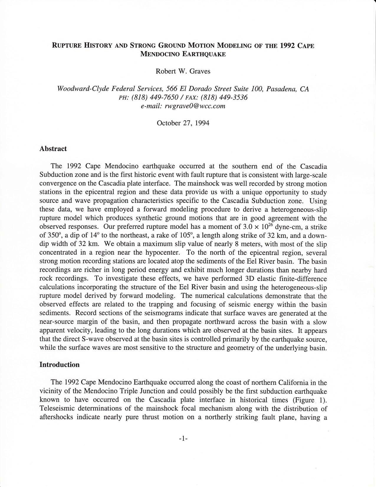
Cape Mendocino Region Model
This manuscript describes some 3D modeling of the Eel River basin which is in the Cape Mendocino region at the northern end of the San Andreas. Robert Graves did this work as part of the development of the 3D FD methodology and published as a USGS external grant report in Graves (1994).
Parkfield Regional Model
Parkfield regional model, published in Thurber et al. (2006). Bounding box corners:
TOP:
35.918339 -121.412085
36.6838908 -120.320581

BOTTOM:
35.0996582 -120.542912
35.86521 -119.45284
The model is fully documented in the supplementary information for the paper Thurber et al (2006).
San Francisco Regional Model
A higher-resolution model for the San Francisco Bay area, published in Thurber et al (2007). It covers a smaller region than our northern California model.
Wasatch Front Model (Utah)
UCVM Utah This is a Utah Geological Survey velocity model for NE Utah, developed by Harold Magistrale and described at wfcvm.
Overview of CVM Models
These posters and presentations may contain information about earlier versions of CVM-H. This information may be useful to some users.
- Computer Science Journal Article describing UCVM Software and Architecture
- Maechling UCVM Overview Presentation 2013 (50Mb ppt)
- Patrick Small UCVM Software Description Presentation 2013 (5Mb ppt)
- Overview of CVM-H 11.2 (1Mb powerpoint file)
- Overview of CVM-H 11.1 (1Mb powerpoint file)
- Andreas Plesch Overview of CVM-H (2008) (7.4Mb powerpoint file)
- CVM-H Poster SCEC Annual Meeting (2008) (1.8Mb pdf file)
- Overview of SCEC Unified Structure Representation (USR) Developments (4.2Mb powerpoint file)
UCVM Software
A software framework has been developed to support a state-wide model. The framework contains a command-line query tool and a C API for querying any supported velocity model.
Coverage Region and Projection
Projection for 2D Maps
The following is the coverage region and projection for the included 2D elevation and Vs30 maps. The entire state of California is included, along with portions of Oregon, Nevada, Arizona, and northern Mexico.
Origin: -129.75 DD, 40.75 DD
Projection: Azimuthal Equidistant (Proj.4 projection string "+proj=aeqd +lat_0=36.0 +lon_0=-120.0 +x_0=0.0 +y_0=0.0")
Rotation Angle: 55.0 D
Dimensions: 1800km x 900km
- UCVM 2D map versus regional CVM coverage areas UCVM 2D Map Boundaries in KML format
- Extremes of UCERF 2.0 ruptures we would like to include (kml)
Statewide Data Sets
DEM
A statewide DEM for the proposed coverage region is included within UCVM. Elevation data has been sampled from USGS NED 1 arcsec dataset (~30 m), and bathymetric data from the NOAA ETOPO1 1' dataset (~1.5 km). This DEM is currently sampled at a resolution of approximately 220m but this may be increased. The elevation data is stored as a fixed resolution Etree for the entire 1800 x 900 km region. The elevation at a particular point is smoothed using bilinear interpolation of the surrounding four elevation octants.

Vs30 Maps
Two statewide Vs30 maps for the proposed coverage region are included within UCVM:
- Wills-Wald Vs30 map (default): Vs30 data for the California landmass has been sampled from the Wills (2006) dataset at approx 0.0002197 D resolution, and out-of-state/ocean areas have been sampled from the Wald (2007) dataset at 0.0083333 D resolution.
- Yong-Wald Vs30 map (optional): Vs30 data for the California landmass has been sampled from the Yong (2011) dataset at approx 0.013 D resolution, and out-of-state/ocean areas have been sampled from the Wald (2007) dataset at 0.0083333 D resolution.
These maps are currently sampled at a resolution of approximately 220m but this may be increased. The Vs30 data is stored as a fixed resolution Etree for the entire 1800 x 900 km region. The Vs30 value at a particular point is smoothed using bilinear interpolation of the surrounding four map octants.

Geotechnical Layer
A statewide GTL for the proposed coverage region is included within UCVM. This is based on the Vs30-derived GTL method developed by Ely (2010). Interpolation between this GTL and the underlying crustal models is accomplished with the interpolation method described in that same publication. The z range over which interpolation is performed is configurable, as is the interpolation method used. The Ely method takes its input Vs30 value from the Vs30 map included within UCVM (described in the previous section).

Additionally, UCVM is able to support any number of other user-defined GTLs. It will combine them in a manner analogous to how the crustal models are combined. Each GTL may also have its own user-defined interpolation function that is used to blend it with the underlying crustal models. If no interpolation method is specified, linear interpolation is assumed.

Hydrology Map
A statewide hydrology map for the proposed coverage region will be included within UCVM. This map will provide the surface elevations of bodies of water such as oceans, lakes, and seas. No source dataset has been identified as of yet. This map will allow water information to be returned when UCVM is queried by elevation.
Documention
The user guide is available at UCVM User Guide.
UCVM Issue Tracking System
Users can report issues, bugs, and request features using the UCVM Trac system. Requires a SCEC login.
UCVM Beyond California
The UCVM code base has no specific dependencies upon the state of California. UCVM may be quickly configured for a new region given digital elevation data, Vs30 data, and one or more velocity models. As a proof of concept, this was done for northern Utah (see UCVM Utah) using the Utah Geological Survery Wasatch Front velocity model.
Future Models to be Integrated
- Central United States CVM
- Allam_Zigone_Ben-Zion_etal_2015
Previous Software Versions
- UCVM 14.3.0
- This version includes CVM-H 14.3, and CVM-S4 California Velocity Models - Released March, 2014. This version is available as a reference only, if needed to reproduce results that used this earlier version. The recommended version is the most recent version available at the top of this page UCVM.
Related Entries
- UCVM User Guide
- UCVM API
- UCVM Visualization
- CVM-H
- CVM-S
- UCVM Utah
- UCVM 15.10.0
- UCVM 14.3.0
- CVM-S5
- CVM-SI
- Community Velocity Model
- Collection of Presentations about CVM-S and CVM-H (56Mb ppt file)
See Also
- BlueWaters Etrees
- Harvard Structural Geology & Earth Resources Group
- Geoff Ely Vs30 geotechnical layer implementation
- Qinya Liu Tomography Research
- GuoQing Lin's Research
- USGS CVM Web Site
- Main Page
- SCEC Home Page
References
- Ely, G., T. H. Jordan, P. Small, P. J. Maechling (2010), A Vs30-derived Near-surface Seismic Velocity Model Abstract S51A-1907, presented at 2010 Fall Meeting, AGU, San Francisco, Calif., 13-17 Dec. [Ely2010-AGU.pdf]
- Graves, R. (1994), Rupture History and Strong Motion Modeling of the 1992 Cape Mendocino Earthquake, USGS External Grant Report
- Lin, G., C. H. Thurber, H. Zhang, E. Hauksson, P. Shearer, F. Waldhauser, T. M. Brocher, and J. Hardebeck (2010), A California statewide three-dimensional seismic velocity model from both absolute and differential Times, Bull. Seism. Soc. Am., 100, in press. supplemental
- Taborda R., López J., O'Hallaron D., Tu T. and Bielak J. (2007), A review of the current approach to CVM-Etrees, SCEC Annual Meeting, Palm Springs, CA, USA, September 8–12. [1]
- Thurber, C., H. Zhang, F. Waldhauser, J. Hardebeck, A. Michael, and D. Eberhart-Phillips (2006), Three-dimensional compressional wavespeed model, earthquake relocations, and focal mechanisms for the Parkfield, California, region, Bull. Seism. Soc. Am., 96, S38-S49, 2006. supplemental
- Thurber, C., T. Brocher, H. Zhang, and V. Langenheim (2007), Three-dimensional P-wave velocity model for the San Francisco Bay region, California, J. Geophys. Res., 112, B07313, doi:10.1029/ 2006JB004682, 2007.
- Thurber, C., H. Zhang, T. Brocher, and V. Langenheim (2009), Regional three-dimensional seismic velocity model of the crust and uppermost mantle of northern California, J.Geophys. Res., 114, B01304, doi:10.1029/2008JB005766, 2009.
- Wald, D. J., and T. I. Allen (2007), Topographic slope as a proxy for seismic site conditions and amplification, Bull. Seism. Soc. Am., 97 (5), 1379-1395, doi:10.1785/0120060267.
- Wills, C. J., and K. B. Clahan (2006), Developing a map of geologically defined site-condition categories for California, Bull. Seism. Soc. Am., 96 (4A), 1483-1501, doi:10.1785/0120050179.
- Yong, A., Hough, S.E., Iwahashi, J., and A. Braverman (2012), A terrain-based site conditions map of California with implications for the contiguous United States, Bull. Seism. Soc. Am., Vol. 102, No. 1, pp. 114–128, February 2012, doi: 10.1785/0120100262.