Difference between revisions of "CyberShake Study 20.5"
| (42 intermediate revisions by the same user not shown) | |||
| Line 1: | Line 1: | ||
| − | CyberShake Study 20.5 is a CyberShake study in Southern California which uses [[Rupture_Variation_Generator_v5.4.2|Graves & Pitarka (2019)]] and includes stochastic high frequencies using the Graves & Pitarka high-frequency module from the SCEC Broadband Platform. | + | CyberShake Study 20.5 is a proposed CyberShake study in Southern California which uses [[Rupture_Variation_Generator_v5.4.2|Graves & Pitarka (2019)]] and includes stochastic high frequencies using the Graves & Pitarka high-frequency module from the SCEC Broadband Platform. |
== RotD code verification == | == RotD code verification == | ||
| − | We performed a verification exercise with the CyberShake RotD code. Christine selected 40 station recordings from Hector Mine, and we calculated PGA and PGV by passing very small periods to the RotD50 code. | + | We performed a verification exercise with the CyberShake RotD code. Christine selected 40 station recordings from Hector Mine (data [[:File:HECTORTest.zip|here]]), and we calculated PGA and PGV by passing very small periods to the RotD50 code. |
| − | Summary results are presented below: | + | Full results of our Hector Mine tests are available [[:File:CyberShake_Hector_comparison.xls|here]]. Summary results are presented below: |
| − | {| | + | {| border="1" cellpadding="3" |
! Metric !! Average absolute percent difference (over 40 stations) | ! Metric !! Average absolute percent difference (over 40 stations) | ||
|- | |- | ||
| Line 26: | Line 26: | ||
|} | |} | ||
| − | Since most of the Hector Mine recordings have small amplitudes compared to CyberShake (PGA=0.02g to 0.3g), we also performed comparisons for 2 sites from Northridge (PGA=0.5g and 0.8g). The calculated PGA values exactly matched those provided from PEER for the Northridge sites. | + | Since most of the Hector Mine recordings have small amplitudes compared to CyberShake (PGA=0.02g to 0.3g), we also performed comparisons for 2 sites from Northridge (PGA=0.5g and 0.8g). The calculated PGA values exactly matched those provided from PEER for the Northridge sites. Input data is available [[:File:NORTHRTest.zip|here]]. Full results are available [[:File:CyberShake_Northridge_comparison.xls|here]]. |
In conclusion, the differences in the PGA results are small -- about the same as the differences we see when moving between systems -- and get smaller as the ground motions increase, so they are unlikely to have any meaningful impact on CyberShake curves. | In conclusion, the differences in the PGA results are small -- about the same as the differences we see when moving between systems -- and get smaller as the ground motions increase, so they are unlikely to have any meaningful impact on CyberShake curves. | ||
| Line 32: | Line 32: | ||
Because the PGV results have such a higher difference than the PGA results, we suspected that the PEER-provided velocity seismograms weren't what PEER used to calculate their PGV. We decided to try integrating the acceleration seismograms ourselves and calculating PGV from those. | Because the PGV results have such a higher difference than the PGA results, we suspected that the PEER-provided velocity seismograms weren't what PEER used to calculate their PGV. We decided to try integrating the acceleration seismograms ourselves and calculating PGV from those. | ||
| − | {| | + | {| border="1" cellpadding="3" |
! Metric !! Average absolute percent difference (over 40 stations) | ! Metric !! Average absolute percent difference (over 40 stations) | ||
|- | |- | ||
! PGV, using period=1e-4 and integrating with left rule | ! PGV, using period=1e-4 and integrating with left rule | ||
| 0.1306% | | 0.1306% | ||
| + | |- | ||
! PGV, using period=1e-4 and integrating with trapezoid rule | ! PGV, using period=1e-4 and integrating with trapezoid rule | ||
| 0.0349% | | 0.0349% | ||
| − | ! PGV, using period=1e-4, trapezoid rule, and using g = 981 cm/s2 | + | |- |
| + | ! PGV, using period=1e-4, trapezoid rule, and using g = 981 cm/s2 | ||
| 0.0% | | 0.0% | ||
|} | |} | ||
| Line 46: | Line 48: | ||
Based on this work, we will use a period of 1e-4 to obtain CyberShake PGA and PGV using the RotD code. | Based on this work, we will use a period of 1e-4 to obtain CyberShake PGA and PGV using the RotD code. | ||
| + | |||
| + | == Impulse modifications == | ||
| + | |||
| + | We discovered that the current impulse used as input to the SGT simulations, which has a tdelay of 1 second (meaning that the peak occurs at t=1 sec), results in artificial truncation of some of the impulse lobes. To correct this, we changed tdelay to 3 seconds in both the impulse generator and the code which populates the SGT headers, so that it is handled correctly during synthesis. This produces more complete impulses, with an integral closer to normalized 1. | ||
| + | |||
| + | {| | ||
| + | | [[File:tdelay_impulse_comparison.png|thumb|600px]] | ||
| + | |} | ||
| + | |||
| + | == Conditional Hypocenter Distributions == | ||
| + | |||
| + | Based on Kevin's dissertation work showing that non-uniform hypocenter distributions can cause significant differences in OEF forecasts, we investigated the effects of conditional hypocenter distributions (CHD) on overall CyberShake results. Images from this work are available [https://github.com/kevinmilner/cybershake-analysis/tree/master/study_15_4/chd_betadist_a10.03_b10.03 here]. | ||
| + | |||
| + | Our conclusion is that, while using a CHD similar to that in Jessica Donovan's thesis can result in changes in long-period hazard up to 20%, we will continue to use a uniform distribution when calculating CyberShake curves. If alternative hypocenter distributions are of interest, the probabilities can always be modified after the fact, but at this point we don't have a clear use case for non-uniform CHD other than general interest. | ||
| + | |||
| + | == Rupture velocity (rvfrac) == | ||
| + | |||
| + | One of the parameters to the rupture generator is rvfrac, indicating what fraction of shear wave speed the rupture velocity is. In past CyberShake runs, we have used a constant 0.8 value for all ruptures. However, varying rvfrac has a big impact on ground motion. Therefore, we investigated the impact of changing rvfrac. | ||
| + | |||
| + | We calculated hazard curves for USC using rvfrac=0.6, 0.7, 0.8, and 0.9. As expected, this has a significant impact on the hazard curves, and the intensity measure distribution: | ||
| + | |||
| + | {| | ||
| + | ! Period !! 2 sec !! 3 sec !! 5 sec !! 10 sec | ||
| + | |- | ||
| + | ! Curve | ||
| + | | [[File:2sec_rvfrac_compare.png|thumb|300px|Comparison of 4 values of rvfrac for site USC, 2 sec RotD50]] | ||
| + | | [[File:3sec_rvfrac_compare.png|thumb|300px|Comparison of 4 values of rvfrac for site USC, 3 sec RotD50]] | ||
| + | | [[File:5sec_rvfrac_compare.png|thumb|300px|Comparison of 4 values of rvfrac for site USC, 5 sec RotD50]] | ||
| + | | [[File:10sec_rvfrac_compare.png|thumb|300px|Comparison of 4 values of rvfrac for site USC, 10 sec RotD50]] | ||
| + | |} | ||
| + | |||
| + | Here are scatterplots of IM values, showing the impact of successive increases in rvfrac on ground motion. | ||
| + | |||
| + | {| | ||
| + | | [[File:0.6_v_0.7_scatter.png|thumb|300px|Comparison of 3 sec RotD50, 0.6 vs 0.7]] | ||
| + | | [[File:0.7_v_0.8_scatter.png|thumb|300px|Comparison of 3 sec RotD50, 0.7 vs 0.8]] | ||
| + | | [[File:0.8_v_0.9_scatter.png|thumb|300px|Comparison of 3 sec RotD50, 0.8 vs 0.9]] | ||
| + | |} | ||
| + | |||
| + | Additionally, we calculated hazard curves using the combined results from all 4 sets of IMs (so that the probability for each rupture is divided over 4 times as many rupture variations). We compared this to hazard curves created by randomly selected an IM for each rupture variation from the 4 sets of IMs. We sampled 5 random curves, along with the the average of these random samples. | ||
| + | |||
| + | {| | ||
| + | ! Period !! 2 sec !! 3 sec !! 5 sec !! 10 sec | ||
| + | |- | ||
| + | ! Curve | ||
| + | | [[File:2sec_rvfrac_random.png|thumb|300px]] | ||
| + | | [[File:3sec_rvfrac_random.png|thumb|300px]] | ||
| + | | [[File:5sec_rvfrac_random.png|thumb|300px]] | ||
| + | | [[File:10sec_rvfrac_random.png|thumb|300px]] | ||
| + | |- | ||
| + | ! Zoomed | ||
| + | | [[File:2sec_rvfrac_random_zoomed.png|thumb|300px]] | ||
| + | | | ||
| + | | | ||
| + | | [[File:10sec_rvfrac_random_zoomed.png|thumb|300px]] | ||
| + | |} | ||
| + | |||
| + | We also tried sampling with 15% from 0.6 and 0.9 and 35% from 0.7 and 0.8. | ||
| + | |||
| + | |||
| + | {| | ||
| + | ! Period !! 2 sec !! 3 sec !! 5 sec !! 10 sec | ||
| + | |- | ||
| + | ! Curve | ||
| + | | [[File:2sec_rvfrac_random_weighted.png|thumb|300px]] | ||
| + | | [[File:3sec_rvfrac_random_weighted.png|thumb|300px]] | ||
| + | | [[File:5sec_rvfrac_random_weighted.png|thumb|300px]] | ||
| + | | [[File:10sec_rvfrac_random_weighted.png|thumb|300px]] | ||
| + | |- | ||
| + | ! Zoomed | ||
| + | | [[File:2sec_rvfrac_random_weighted_zoomed.png|thumb|300px]] | ||
| + | | | ||
| + | | | ||
| + | | [[File:10sec_rvfrac_random_weighted_zoomed.png|thumb|300px]] | ||
| + | |} | ||
| + | |||
| + | == Velocity Model == | ||
| + | |||
| + | Some locations, especially in CVM-S4.26.M01, have a sharp transition between the velocity at the surface and the velocity a few meters down. For example, at site PAS (34.14826, -118.17119): | ||
| + | |||
| + | [[File:PAS_Vs_profile.png|right]] | ||
| + | |||
| + | {| | ||
| + | ! Depth (m) !! Vs | ||
| + | |- | ||
| + | | 0.0 || 309.048 | ||
| + | |- | ||
| + | | 1.0 || 309.048 | ||
| + | |- | ||
| + | | 2.0 || 370.518 | ||
| + | |- | ||
| + | | 3.0 || 370.518 | ||
| + | |- | ||
| + | | 5.0 || 663.146 | ||
| + | |- | ||
| + | | 10.0 || 1301.360 | ||
| + | |- | ||
| + | | 15.0 || 1334.606 | ||
| + | |- | ||
| + | | 20.0 || 1360.615 | ||
| + | |- | ||
| + | | 25.0 || 1378.660 | ||
| + | |- | ||
| + | | 30.0 || 1341.732 | ||
| + | |- | ||
| + | | 50.0 || 1405.032 | ||
| + | |- | ||
| + | | 75.0 || 1449.194 | ||
| + | |- | ||
| + | | 100.0 || 1500.181 | ||
| + | |} | ||
| + | |||
| + | The surface mesh point is supposed to represent the velocities from 0 to h/2, where h is the grid spacing. This is 50m for Study 20.5. But for a site like PAS Vs=309 is a poor representative value. Vs30, calculated using a slowness average, is 839, and Vs50 is 993. | ||
| + | |||
| + | Therefore, we have added the capability of using an arbitrary depth, represented as a fraction of a grid point, when querying UCVM to populate surface mesh points. | ||
| + | |||
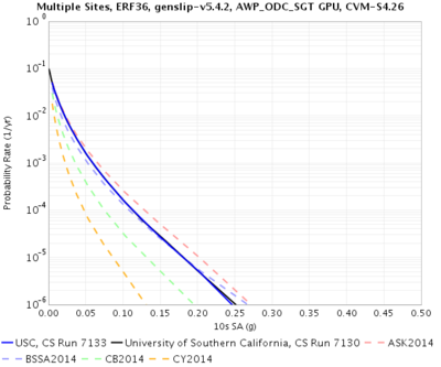
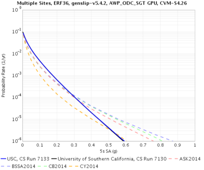
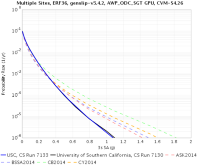
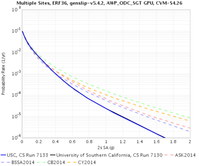
| + | Here is a comparison of hazard curves for site USC using z=0 to populate the mesh points (Run 7130, in <span style="color:blue">blue</span>), and z=h/4 (25m) (Run 7133, black). Since we are slightly increasing the velocity of the surface point, we would expect slightly lower hazard, which is what we see. | ||
| + | |||
| + | {| border="1" | ||
| + | ! 10 sec !! 5 sec !! 3 sec !! 2 sec | ||
| + | |- | ||
| + | | [[File:USC_7130_v_7133_RotD50_10sec.png|thumb|400px]] | ||
| + | | [[File:USC_7130_v_7133_RotD50_5sec.png|thumb|400px]] | ||
| + | | [[File:USC_7130_v_7133_RotD50_3sec.png|thumb|400px]] | ||
| + | | [[File:USC_7130_v_7133_RotD50_2sec.png|thumb|400px]] | ||
| + | |} | ||
== Output Data Products == | == Output Data Products == | ||
| Line 51: | Line 179: | ||
=== Seismograms === | === Seismograms === | ||
| − | * Deterministic (dt=0.05, nt= | + | * Deterministic (dt=0.05, nt=10000) |
| − | * Broadband (dt=0.01, nt= | + | * Broadband (dt=0.01, nt=50000) |
=== Intensity Measures === | === Intensity Measures === | ||
| Line 110: | Line 238: | ||
10, 5, 3, 2, 1, 0.5, 0.3, 0.2, 0.1 sec | 10, 5, 3, 2, 1, 0.5, 0.3, 0.2, 0.1 sec | ||
| + | |||
| + | == Vs values == | ||
| + | |||
| + | A number of Vs-derived values are used in various parts of the broadband CyberShake code, and we have made some changes in preparation for this study. | ||
| + | |||
| + | For some locations (infamously, Pasadena), UCVM has much lower velocities in the top few meters than deeper down. Since the velocity value of the top mesh point is really used to represent the entire layer from the surface to half the mesh spacing (so for 100m mesh spacing, the top 50m), we have decided to start querying UCVM at one-fourth of the mesh spacing (h/4) and use that value to populate the top mesh point (25m, for 100m spacing). | ||
| + | |||
| + | In an effort to standardize and be clear with users about where various Vs proxies come from, we decided to define the following values to be stored in the database. | ||
| + | |||
| + | *Model_Vs30. This is calculated from UCVM using a slowness average. The 30 points in the interval [0.5, 29.5] at 1m increments are queried and slowness-averaged to obtain this value. We do not plan to use it directly in calculations, but rather provide it for reference. | ||
| + | *Mesh_Vsitop. In the past we have stored Vs at the surface mesh point at the CyberShake site, but we have modified this column into something more general. Moving forward, we will still use the value of the surface mesh point, but as mentioned above, this will now be obtained from UCVM by querying at depth h/4 (and of course have the Vs floor and smoothing applied). We also added a metadata table to the database to track how this value is calculated. | ||
| + | *Wills_Vs30. Value from Wills (2015). | ||
| + | *Target_Vs30. This is intended to be the Vs30 value used when doing GMPE comparisons and in broadband calculations. We would like to use the approach of Thompson et al. (2018), as it includes measurements, but since there are some bullseye effects in the San Gabriels due to the smoothing approach, we are going to hold off until Thompson's new map is released. | ||
| + | *Vref_eff. This is the effective Vref used in broadband CyberShake calculations. A metadata table was added so we can track what algorithm is used. The current approach is outlined [[CyberShake_Study_15.12#Vs_values_v3.0 | here]]. | ||
| + | |||
| + | We also identified which Vs values should be used as inputs to the broadband codes. | ||
| + | |||
| + | In the high-frequency site response: | ||
| + | *vref = 500.0 (this is dependent on the 1D velocity model used). | ||
| + | *vsite = Target_Vs30, as outlined above. | ||
| + | *vpga = vref | ||
| + | |||
| + | In the low-frequency site response: | ||
| + | *vref = Vref_eff | ||
| + | *vsite = Target_Vs30 | ||
| + | *vpga = high-frequency vpga | ||
Latest revision as of 19:48, 8 July 2022
CyberShake Study 20.5 is a proposed CyberShake study in Southern California which uses Graves & Pitarka (2019) and includes stochastic high frequencies using the Graves & Pitarka high-frequency module from the SCEC Broadband Platform.
Contents
RotD code verification
We performed a verification exercise with the CyberShake RotD code. Christine selected 40 station recordings from Hector Mine (data here), and we calculated PGA and PGV by passing very small periods to the RotD50 code.
Full results of our Hector Mine tests are available here. Summary results are presented below:
| Metric | Average absolute percent difference (over 40 stations) |
|---|---|
| PGA, using period=1e-3 | 0.0165% |
| PGA, using period=1e-4 | 0.0118% |
| PGA, using period=1e-5 | 0.0118% |
| PGV, using period=1e-3 | 0.532% |
| PGV, using period=1e-4 | 0.526% |
Since most of the Hector Mine recordings have small amplitudes compared to CyberShake (PGA=0.02g to 0.3g), we also performed comparisons for 2 sites from Northridge (PGA=0.5g and 0.8g). The calculated PGA values exactly matched those provided from PEER for the Northridge sites. Input data is available here. Full results are available here.
In conclusion, the differences in the PGA results are small -- about the same as the differences we see when moving between systems -- and get smaller as the ground motions increase, so they are unlikely to have any meaningful impact on CyberShake curves.
Because the PGV results have such a higher difference than the PGA results, we suspected that the PEER-provided velocity seismograms weren't what PEER used to calculate their PGV. We decided to try integrating the acceleration seismograms ourselves and calculating PGV from those.
| Metric | Average absolute percent difference (over 40 stations) |
|---|---|
| PGV, using period=1e-4 and integrating with left rule | 0.1306% |
| PGV, using period=1e-4 and integrating with trapezoid rule | 0.0349% |
| PGV, using period=1e-4, trapezoid rule, and using g = 981 cm/s2 | 0.0% |
This confirms that the RotD code is working correctly, and the issues with PGV agreement are because the PEER PGV values aren't actually calculated from their velocity seismograms.
Based on this work, we will use a period of 1e-4 to obtain CyberShake PGA and PGV using the RotD code.
Impulse modifications
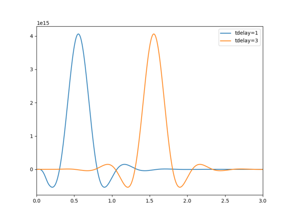
We discovered that the current impulse used as input to the SGT simulations, which has a tdelay of 1 second (meaning that the peak occurs at t=1 sec), results in artificial truncation of some of the impulse lobes. To correct this, we changed tdelay to 3 seconds in both the impulse generator and the code which populates the SGT headers, so that it is handled correctly during synthesis. This produces more complete impulses, with an integral closer to normalized 1.
Conditional Hypocenter Distributions
Based on Kevin's dissertation work showing that non-uniform hypocenter distributions can cause significant differences in OEF forecasts, we investigated the effects of conditional hypocenter distributions (CHD) on overall CyberShake results. Images from this work are available here.
Our conclusion is that, while using a CHD similar to that in Jessica Donovan's thesis can result in changes in long-period hazard up to 20%, we will continue to use a uniform distribution when calculating CyberShake curves. If alternative hypocenter distributions are of interest, the probabilities can always be modified after the fact, but at this point we don't have a clear use case for non-uniform CHD other than general interest.
Rupture velocity (rvfrac)
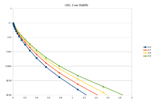
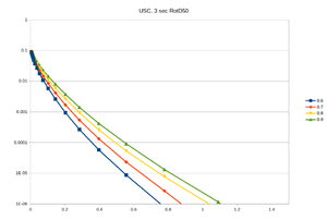
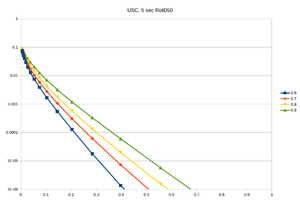
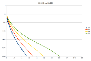
One of the parameters to the rupture generator is rvfrac, indicating what fraction of shear wave speed the rupture velocity is. In past CyberShake runs, we have used a constant 0.8 value for all ruptures. However, varying rvfrac has a big impact on ground motion. Therefore, we investigated the impact of changing rvfrac.
We calculated hazard curves for USC using rvfrac=0.6, 0.7, 0.8, and 0.9. As expected, this has a significant impact on the hazard curves, and the intensity measure distribution:
| Period | 2 sec | 3 sec | 5 sec | 10 sec |
|---|---|---|---|---|
| Curve |
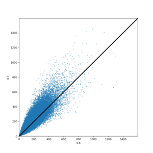
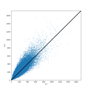
Here are scatterplots of IM values, showing the impact of successive increases in rvfrac on ground motion.
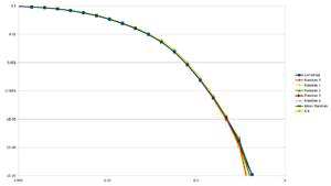
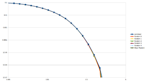
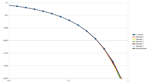
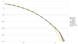
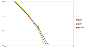
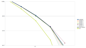
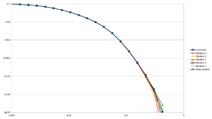
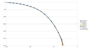
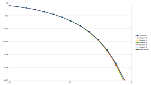
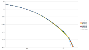
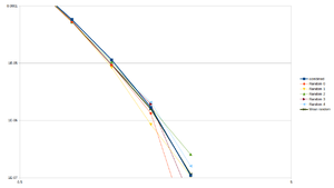
Additionally, we calculated hazard curves using the combined results from all 4 sets of IMs (so that the probability for each rupture is divided over 4 times as many rupture variations). We compared this to hazard curves created by randomly selected an IM for each rupture variation from the 4 sets of IMs. We sampled 5 random curves, along with the the average of these random samples.
| Period | 2 sec | 3 sec | 5 sec | 10 sec |
|---|---|---|---|---|
| Curve | ||||
| Zoomed |
We also tried sampling with 15% from 0.6 and 0.9 and 35% from 0.7 and 0.8.
| Period | 2 sec | 3 sec | 5 sec | 10 sec |
|---|---|---|---|---|
| Curve | ||||
| Zoomed |
Velocity Model
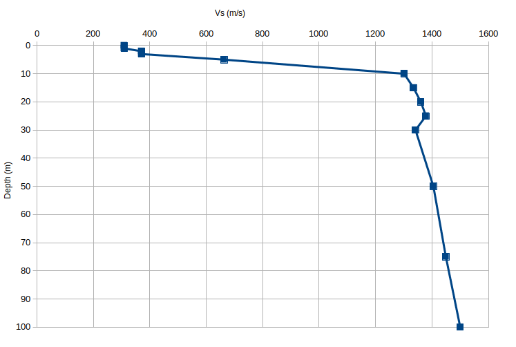
Some locations, especially in CVM-S4.26.M01, have a sharp transition between the velocity at the surface and the velocity a few meters down. For example, at site PAS (34.14826, -118.17119):
| Depth (m) | Vs |
|---|---|
| 0.0 | 309.048 |
| 1.0 | 309.048 |
| 2.0 | 370.518 |
| 3.0 | 370.518 |
| 5.0 | 663.146 |
| 10.0 | 1301.360 |
| 15.0 | 1334.606 |
| 20.0 | 1360.615 |
| 25.0 | 1378.660 |
| 30.0 | 1341.732 |
| 50.0 | 1405.032 |
| 75.0 | 1449.194 |
| 100.0 | 1500.181 |
The surface mesh point is supposed to represent the velocities from 0 to h/2, where h is the grid spacing. This is 50m for Study 20.5. But for a site like PAS Vs=309 is a poor representative value. Vs30, calculated using a slowness average, is 839, and Vs50 is 993.
Therefore, we have added the capability of using an arbitrary depth, represented as a fraction of a grid point, when querying UCVM to populate surface mesh points.
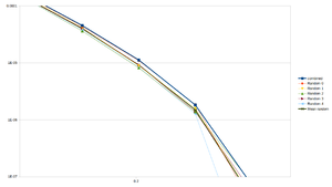
Here is a comparison of hazard curves for site USC using z=0 to populate the mesh points (Run 7130, in blue), and z=h/4 (25m) (Run 7133, black). Since we are slightly increasing the velocity of the surface point, we would expect slightly lower hazard, which is what we see.
| 10 sec | 5 sec | 3 sec | 2 sec |
|---|---|---|---|
Output Data Products
Seismograms
- Deterministic (dt=0.05, nt=10000)
- Broadband (dt=0.01, nt=50000)
Intensity Measures
Values for database
We will calculate and store the following intensity measures in the database (all PSA values are for 5% damping).
For deterministic seismograms (as simulated):
- Store RotD50, RotD100 at the following 7 periods:
10, 7.5, 5, 4, 3, 2, 1
For broadband seismograms (include minor site effects modifications):
- Store RotD50, RotD100 in the database at the following 21 periods:
10, 7.5, 5, 4, 3, 2, 1, 0.75, 0.5, 0.4, 0.3, 0.2, 0.1, 0.075, 0.05, 0.04, 0.03, 0.02, 0.01, PGA, PGV
Durations
Values for database
We will store the following durations in the database for broadband seismograms:
- Acceleration significant duration based on Arias intensity at 5-75% and 5-95%, for both X and Y
Hazard Curves
We will calculate deterministic hazard curves at the following frequencies:
10, 5, 3, 2 sec
We will calculate broadband hazard curves at the following frequencies:
10, 5, 3, 2, 1, 0.5, 0.3, 0.2, 0.1 sec
Vs values
A number of Vs-derived values are used in various parts of the broadband CyberShake code, and we have made some changes in preparation for this study.
For some locations (infamously, Pasadena), UCVM has much lower velocities in the top few meters than deeper down. Since the velocity value of the top mesh point is really used to represent the entire layer from the surface to half the mesh spacing (so for 100m mesh spacing, the top 50m), we have decided to start querying UCVM at one-fourth of the mesh spacing (h/4) and use that value to populate the top mesh point (25m, for 100m spacing).
In an effort to standardize and be clear with users about where various Vs proxies come from, we decided to define the following values to be stored in the database.
- Model_Vs30. This is calculated from UCVM using a slowness average. The 30 points in the interval [0.5, 29.5] at 1m increments are queried and slowness-averaged to obtain this value. We do not plan to use it directly in calculations, but rather provide it for reference.
- Mesh_Vsitop. In the past we have stored Vs at the surface mesh point at the CyberShake site, but we have modified this column into something more general. Moving forward, we will still use the value of the surface mesh point, but as mentioned above, this will now be obtained from UCVM by querying at depth h/4 (and of course have the Vs floor and smoothing applied). We also added a metadata table to the database to track how this value is calculated.
- Wills_Vs30. Value from Wills (2015).
- Target_Vs30. This is intended to be the Vs30 value used when doing GMPE comparisons and in broadband calculations. We would like to use the approach of Thompson et al. (2018), as it includes measurements, but since there are some bullseye effects in the San Gabriels due to the smoothing approach, we are going to hold off until Thompson's new map is released.
- Vref_eff. This is the effective Vref used in broadband CyberShake calculations. A metadata table was added so we can track what algorithm is used. The current approach is outlined here.
We also identified which Vs values should be used as inputs to the broadband codes.
In the high-frequency site response:
- vref = 500.0 (this is dependent on the 1D velocity model used).
- vsite = Target_Vs30, as outlined above.
- vpga = vref
In the low-frequency site response:
- vref = Vref_eff
- vsite = Target_Vs30
- vpga = high-frequency vpga
